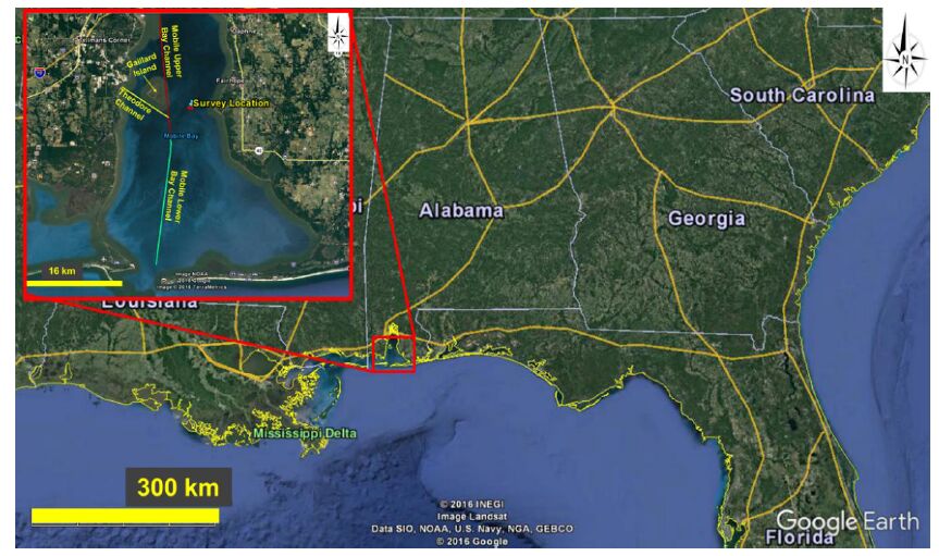
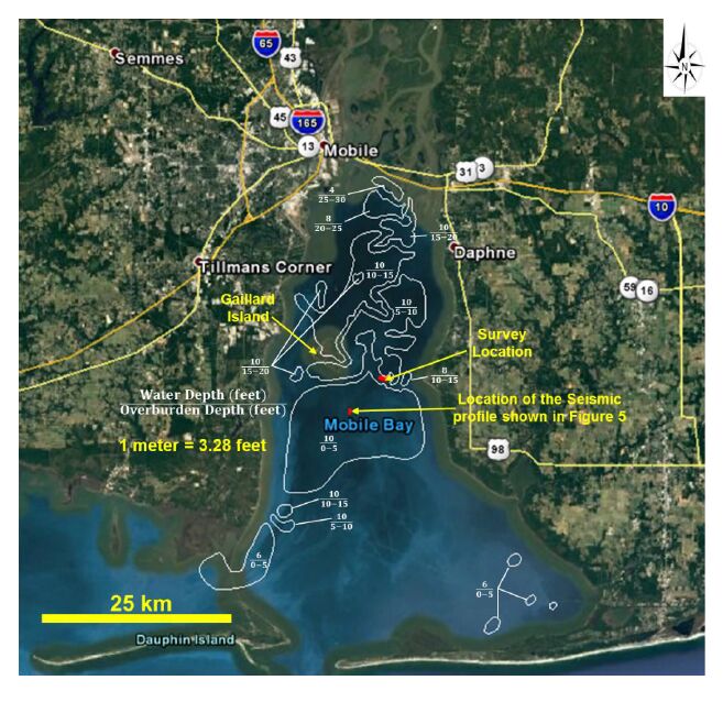
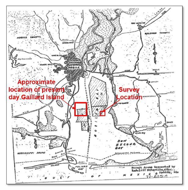
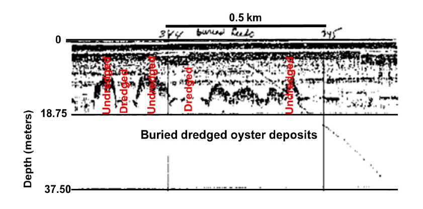
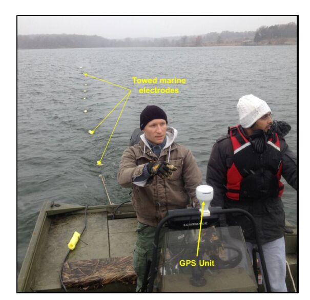
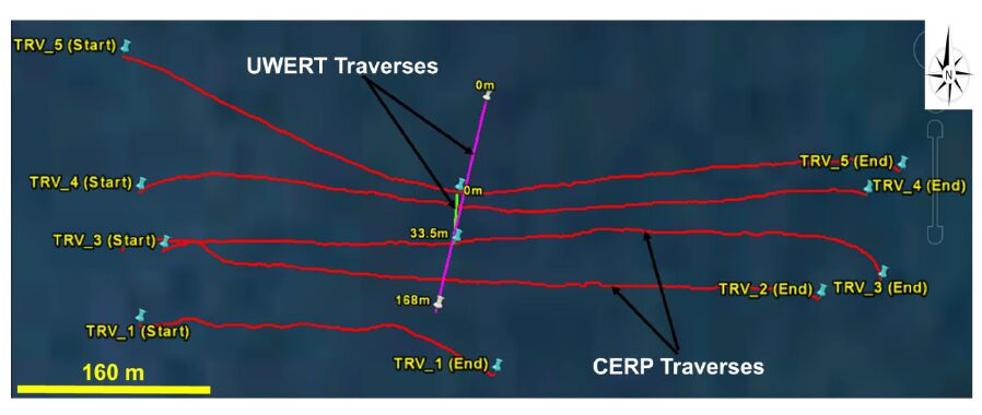
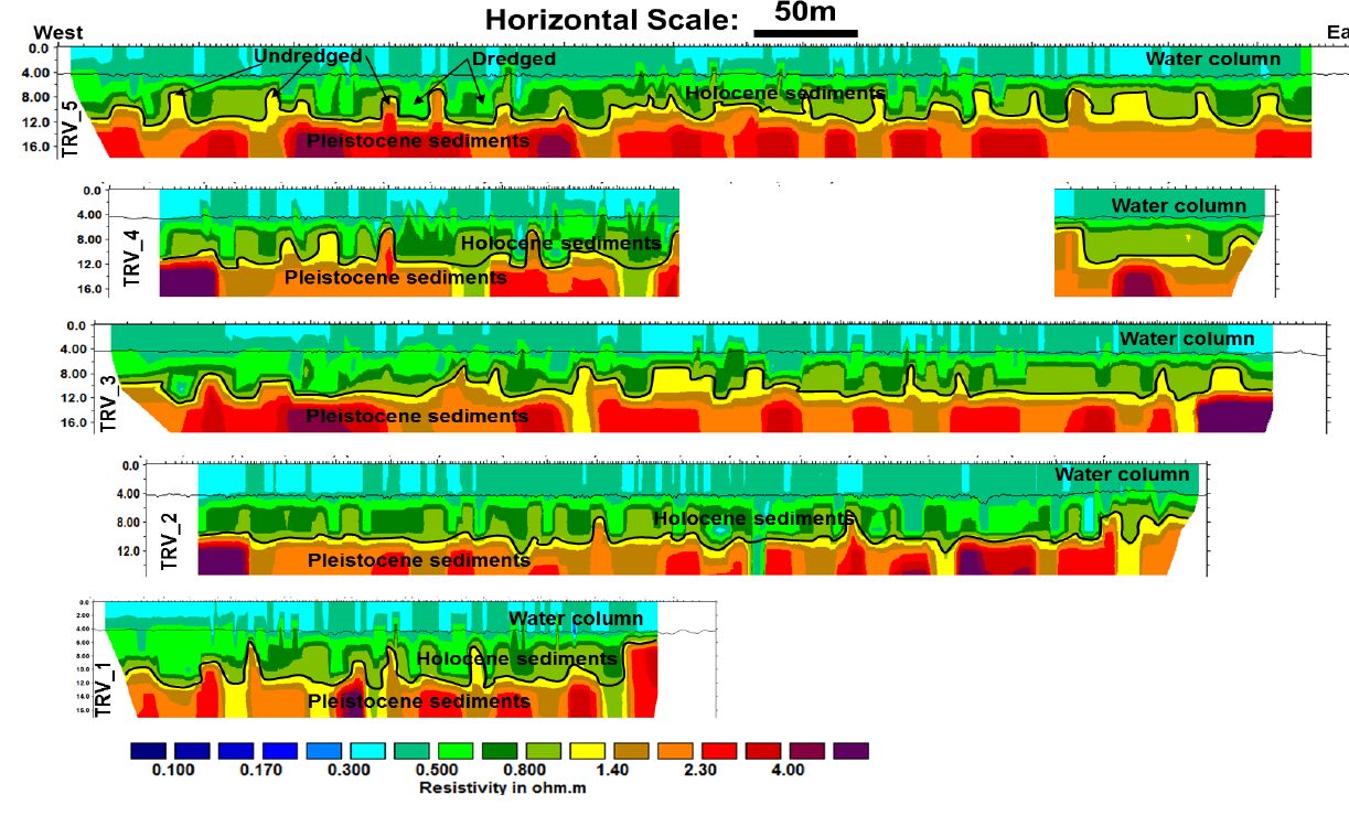
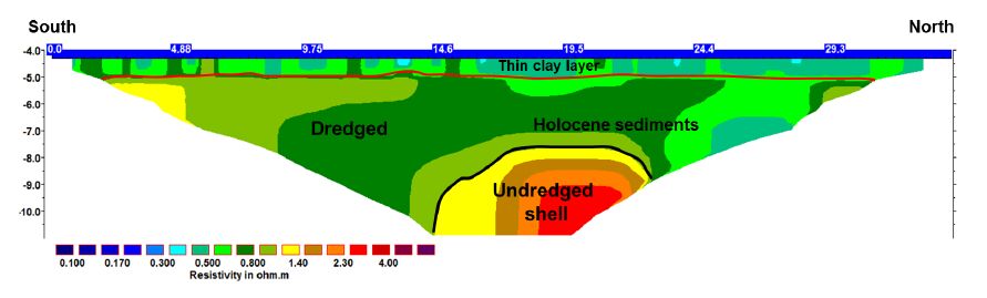
The need for disposing materials dredged from ship channels is a common problem in bays and lagoons. This study is aimed at investigating the suitability of scour features produced by dredging oyster shell deposits in Mobile Bay, Alabama, to dispose excavated channel material. A study area approximately 740 by 280 m lying about 5 km east of Gaillard Island was surveyed using underwater electrical resistivity tomography (UWERT) and continuous electrical resistivity profiling (CERP) tools. The geophysical survey was conducted with the intent to map scour features created by oyster shell dredging activities in the bay between 1947 and 1982. The geoelectrical surveys show that oyster beds are characterized by high resistivity values greater than 1.1 ohm.m while infilled dredge cuts show lower resistivity, generally from 0.6 to 1.1 ohm.m. The difference in resistivity mainly reflects the lithology and the consolidation of the shallow sediments: consolidated silty clay and sandy sediments rich in oyster shell deposits (with less clay content) overlying unconsolidated clayey materials infilling the scours. Results show that most of the infilled dredge cuts are mostly distributed in the north-south direction. Considering that the scours are generally up to 6 m deep across the survey location, it is estimated that about 0.8 million cubic meters of oyster shells and overlying strata were dredged from the survey location.
Citation: Stanley C. Nwokebuihe, Evgeniy Torgashov, Adel Elkrry, Neil Anderson. Characterization of Dredged Oyster Shell Deposits at Mobile Bay, Alabama Using Geophysical Methods[J]. AIMS Geosciences, 2016, 2(4): 401-412. doi: 10.3934/geosci.2016.4.401
The need for disposing materials dredged from ship channels is a common problem in bays and lagoons. This study is aimed at investigating the suitability of scour features produced by dredging oyster shell deposits in Mobile Bay, Alabama, to dispose excavated channel material. A study area approximately 740 by 280 m lying about 5 km east of Gaillard Island was surveyed using underwater electrical resistivity tomography (UWERT) and continuous electrical resistivity profiling (CERP) tools. The geophysical survey was conducted with the intent to map scour features created by oyster shell dredging activities in the bay between 1947 and 1982. The geoelectrical surveys show that oyster beds are characterized by high resistivity values greater than 1.1 ohm.m while infilled dredge cuts show lower resistivity, generally from 0.6 to 1.1 ohm.m. The difference in resistivity mainly reflects the lithology and the consolidation of the shallow sediments: consolidated silty clay and sandy sediments rich in oyster shell deposits (with less clay content) overlying unconsolidated clayey materials infilling the scours. Results show that most of the infilled dredge cuts are mostly distributed in the north-south direction. Considering that the scours are generally up to 6 m deep across the survey location, it is estimated that about 0.8 million cubic meters of oyster shells and overlying strata were dredged from the survey location.

| [1] | May EB (1971) A survey of the oyster and the oyster shell resources of Alabama. Mar Resour Bull 4:1-53. |
| [2] | Lovelace N, Parsons L, Lovelace N, et al (2015) Beneficial Use of Dredged Material to Fill Holes from Oyster Shell Mining in Mobile Bay. FY 16 Regional Sediment Management-Engineering with Nature In-Progress Review Duck, North Carolina May 17-19. |
| [3] | Teatini P, Tosi L, Viezzoli A, et al (2010) Driving the modeling of saltwater intrusion at the Venice coastland (Italy) by ground-based, water-, and air-borne geophysical investigations. World Environ Water Resour Congr 371: 1146-1155. |
| [4] |
Vardy ME, Pinson LJW, Bull JM, et al (2010) 3D seismic imaging of buried Younger Dryas mass movement flows: Lake Windermere, UK. Geomorphol 118: 176-187. doi: 10.1016/j.geomorph.2009.12.017

|
| [5] | Ryan JJ and Goodell HG (1972) Marine geology and estuarine history of Mobile Bay, Alabama. In Environmental Framework of Coastal Plain Estuaries. Geol Soc Am Mem 47: 517-554. |
| [6] | Kindinger J (2016) Evolution and History of Incised Valleys: The Mobile Bay Model: USGS Fact Sheet; Retrieved from: http://pubs.usgs.gov/fs/incised-valleys/. |
| [7] | May EB (1976) Holocene sediments of Mobile Bay, Alabama. Alabama Marine Resources Laboratory. |
| [8] | Mars JC, Shultz AW, Schroeder WW (1992) Stratigraphy and Holocene evolution of Mobile Bay in southwestern Alabama. Gulf Coast Assoc Geol Soc, Trans 42: 529-542. |
| [9] | Agiusa.com (2015) Retrieved from: https://www.agiusa.com/supersting-wi-fi. |
| [10] | Lowrance.com, 2014. Available from: http://www.lowrance.com/en-US/. |
| [11] | Geotomosoft.com, 2014. Retrieved from: http://www.geotomosoft.com/. |
| [12] | Brande S, Dinger JS, McAnnally CW, et al (1983) Seismic Survey of Mississippi Sound, Mississippi, and Mobile Bay, Alabama. Retrieved from: http://nsgl.gso.uri.edu/masgc/masgcw81001/masgcw81001_part6.pdf. |


Figures(10)

Stanley C. Nwokebuihe, Evgeniy Torgashov, Adel Elkrry, Neil Anderson. Characterization of Dredged Oyster Shell Deposits at Mobile Bay, Alabama Using Geophysical Methods[J]. AIMS Geosciences, 2016, 2(4): 401-412. doi: 10.3934/geosci.2016.4.401


 DownLoad: