Geospatial analysis of impact on evacuation routes and urban areas in South Texas due to flood events

Layda B. Spor Leal; Jungseok Ho; Sara Davila; Layda B. Spor Leal; Jungseok Ho; Sara Davila

doi:10.3934/urs.2023002

Urban Resilience and Sustainability

2023, Volume 1, Issue 1: 20-36. doi: 10.3934/urs.2023002

Previous Article Next Article

Research article Special Issues

Geospatial analysis of impact on evacuation routes and urban areas in South Texas due to flood events

Department of Civil Engineering, University of Texas Rio Grande Valley, TX 78539, USA

Received: 03 August 2022 Revised: 18 October 2022 Accepted: 28 October 2022 Published: 03 November 2022

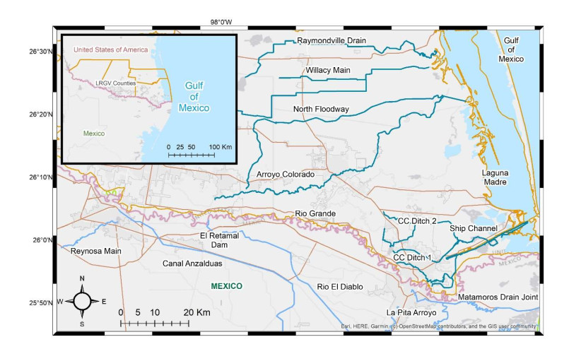
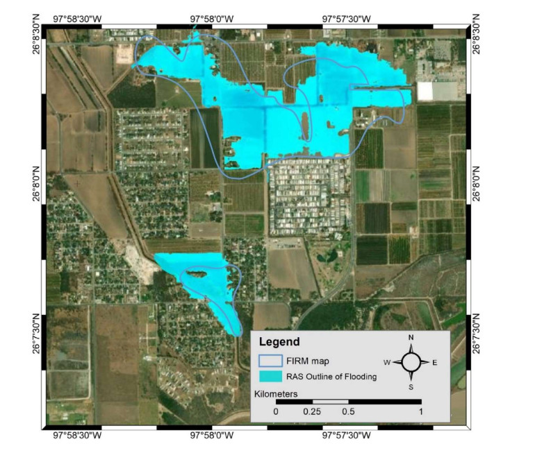
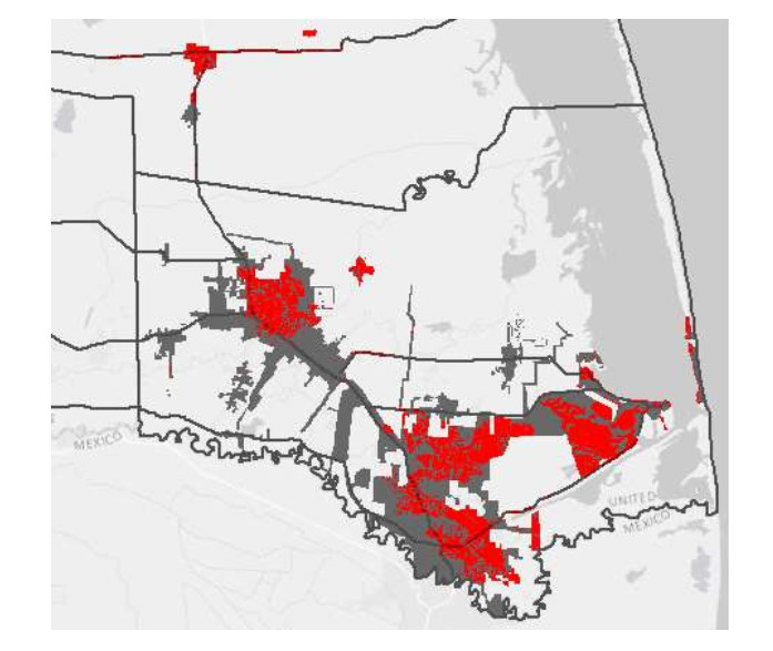
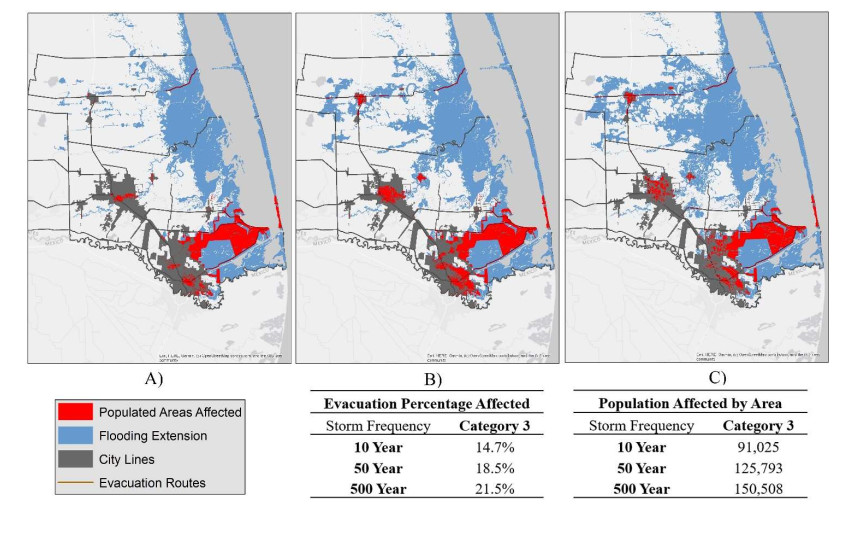
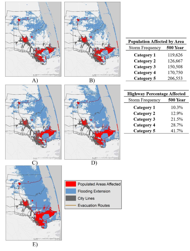
The Lower Rio Grande Valley has historically faced a variety of hurricanes and tropical storms that have led to sever flooding. As a consequence, waves of mass evacuation of the local population with the means of transportation occur frequently. While evacuation is encouraged in some cases of disaster, the routing is not always available as water takes to roads and drainage capacities are overwhelmed. In order to dissert the most appropriate evacuation routes, it is necessary to analyze the areas that will be affected in the future based on urban locations, elevation, and historical information. This project utilizes a semi-coupled hydrodynamic modeling approach that combines the overall spectrum of hurricane storm surge and rainfall induced flooding. The combination of models provide data that can be analyzed with Geographical Information Systems to illustrate the severity of flooding. This analysis can be used to denote the location of the affected evacuation routes and an estimation of population affected in various storm scenarios. The estimated results of this project can be used to not only plan future evacuation routes but denote what areas will possibly require road maintenance after certain flooding scenarios.
- emergency evacuation route,
- affected highway coverage and population,
- coastal hurricane storm surge,
- South Texas
Citation: Layda B. Spor Leal, Jungseok Ho, Sara Davila. Geospatial analysis of impact on evacuation routes and urban areas in South Texas due to flood events[J]. Urban Resilience and Sustainability, 2023, 1(1): 20-36. doi: 10.3934/urs.2023002

Related Papers:

Abstract

The Lower Rio Grande Valley has historically faced a variety of hurricanes and tropical storms that have led to sever flooding. As a consequence, waves of mass evacuation of the local population with the means of transportation occur frequently. While evacuation is encouraged in some cases of disaster, the routing is not always available as water takes to roads and drainage capacities are overwhelmed. In order to dissert the most appropriate evacuation routes, it is necessary to analyze the areas that will be affected in the future based on urban locations, elevation, and historical information. This project utilizes a semi-coupled hydrodynamic modeling approach that combines the overall spectrum of hurricane storm surge and rainfall induced flooding. The combination of models provide data that can be analyzed with Geographical Information Systems to illustrate the severity of flooding. This analysis can be used to denote the location of the affected evacuation routes and an estimation of population affected in various storm scenarios. The estimated results of this project can be used to not only plan future evacuation routes but denote what areas will possibly require road maintenance after certain flooding scenarios.

References

[1]	David Vigness, Mark Odintz, Rio Grande Valley. Texas State Historical Association, 1952. Available from: https://www.tshaonline.org/handbook/entries/rio-grande-valley.
[2]	Office of Emergency Management, Hurricane Preparedness. The University of Texas Rio Grande Valley. Available from: https://www.utrgv.edu/emergencymanagement/get-prepared/hurricane/index.html.
[3]	US Department of Commerce, Flood Safety Awareness for the Lower Rio Grande Valley. NOAA National Weather Service, 2020. Available from: https://www.weather.gov/bro/floodsafety.
[4]	Zerger A (2022) Examining GIS decision utility for natural hazard risk modelling. Environ Model Softw, 17: 287–294. https://doi.org/10.1016/S1364-8152(01)00071-8 doi: 10.1016/S1364-8152(01)00071-8
[5]	Zhang H, Zhang M, Zhang C, et al. (2021) Formulating a GIS-based geometric design quality assessment model for Mountain highways. Accid Anal Prev 157: 106172. https://doi.org/10.1016/j.aap.2021.106172. doi: 10.1016/j.aap.2021.106172
[6]	Unidos Contra la Diabetes, 2022 Demographics. RGV Health Connect, 2022. Available from: https://www.rgvhealthconnect.org/demographicdata?id=281259§ionId=935.
[7]	Lysaniuk B, Cely-García MF, Giraldo M, et al. (2021) Using GIS to estimate population at risk because of residence proximity to asbestos, processing facilities in Colombia. Int J Environ Res Public Health 18: 13297. https://doi.org/10.3390/ijerph182413297 doi: 10.3390/ijerph182413297
[8]	Ozcelik C, Gorokhovich Y, Doocy S (2012) Storm surge modelling with geographic information systems: Estimating areas and population affected by cyclone Nargis. Int J Climat 32: 95–107. https://doi.org/10.1002/joc.2252 doi: 10.1002/joc.2252
[9]	Texas Department of Transportation, Hurricane Evacuation Routes. Texas Department of Transportation, 2021. Available from: https://ftp.txdot.gov/pub/txdot-info/trv/hurricane/rgv-evacuation.pdf.
[10]	Hu X, Wang X, Zheng N, et al. (2021) Experimental investigation of moisture sensitivity and damage evolution of porous asphalt mixtures. Materials 14: 7151. https://doi.org/10.3390/ma14237151 doi: 10.3390/ma14237151
[11]	U.S. Army Corps of Engineers, US Army Corps of Engineers Hydrologic Engineering Center. Available from: https://www.hec.usace.army.mil/software/hec-hms/.
[12]	Brunner GW (2016). HEC-RAS River analysis system, 2D modeling user's manual version 5.0. US Army Corps of Engineers, Hydrologic Engineering Center.
[13]	Sebastian A, Proft J, Dietrich JC, et al. (2014). Characterizing hurricane storm surge behavior in galveston bay using the SWAN+ADCIRC model. Coast Eng 88: 171–181. https://doi.org/10.1016/j.coastaleng.2014.03.002 doi: 10.1016/j.coastaleng.2014.03.002
[14]	Roth D (2010) Texas Hurricane History, National Weather Service. Available from: https://weather.gov/media/lch/events/txhurricanehistory.pdf.
[15]	Davila SE, Garza A, Ho J (2018) Development of hurricane storm surge model to predict coastal highway inundation for South Texas. Int J Interdiscip Cult Stud 6: 522–527. https://doi: 10.3934/geosci.2020016 doi: 10.3934/geosci.2020016
[16]	Nunez C (2019) Here's how hurricanes form—and why they're so destructive. National Geographic. Available from: https://www.nationalgeographic.com/environment/natural-disasters/hurricanes/
[17]	Hydrometeorological Design Studies Center, The Precipitation Frequency Data Server (PFDS). National Weather Service, NOAA. Available from: https://hdsc.nws.noaa.gov/hdsc/pfds.
[18]	Water Science School, The 100-Year Flood Completed. U.S. Geological Survey. USGS, 2018. Available from: https://www.usgs.gov/special-topics/water-science-school/science/100-year-flood.
[19]	Shao W, Su X, Lu J, et al. (2021) The application of big data in the analysis of the impact of urban floods: a case study of Qianshan River Basin. Journal of Physics: Conference Series 1995: 012061. https://doi.org/10.1088/1742-6596/1955/1/012061. doi: 10.1088/1742-6596/1955/1/012061
[20]	US Department of Commerce, Worse than Dolly? Widespread flooding eviscerates drought; impacts entire Rio Grande Valley June 18-22, 2018. NOAA National Weather Service, 2021. Available from: https://www.weather.gov/bro/2018event_greatjuneflood.
[21]	Nancy Houston (2006) Using highways during evacuation operations for events with advance notice, Washington D. C: U.S. Department of Transportation.
[22]	Reyna AL (2022) Hydrologic modeling study to determine hydrologic impact of Resacas on the Lower Laguna Madre watershed, Texas: The University of Texas.

Reader Comments

Your name:*

Email:*
© 2023 the Author(s), licensee AIMS Press. This is an open access article distributed under the terms of the Creative Commons Attribution License (http://creativecommons.org/licenses/by/4.0)