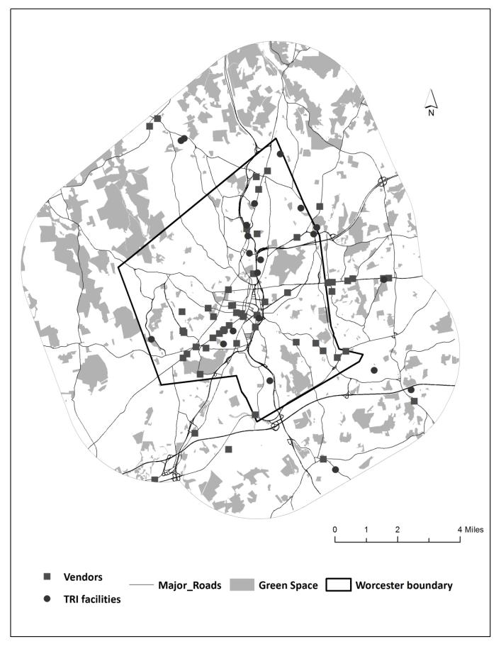
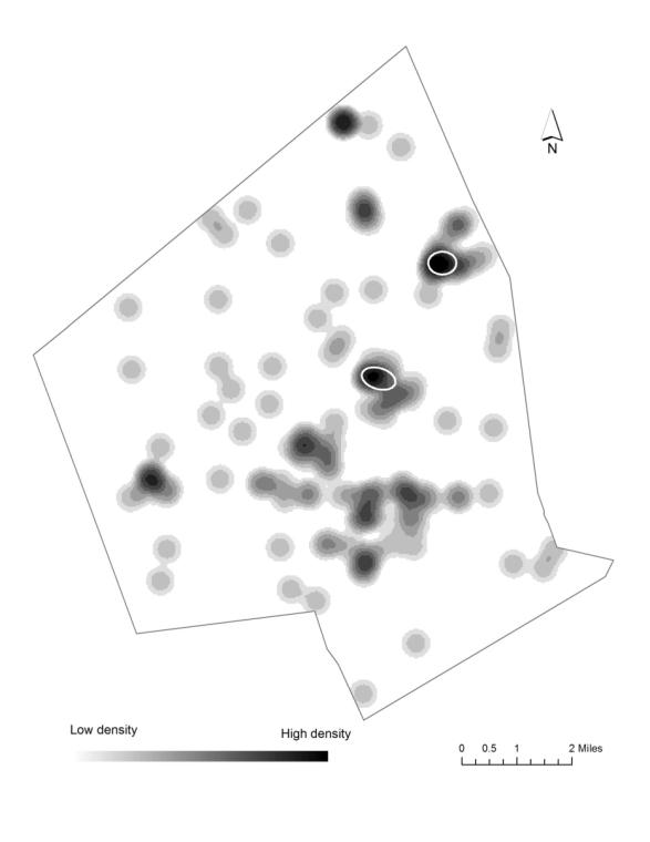
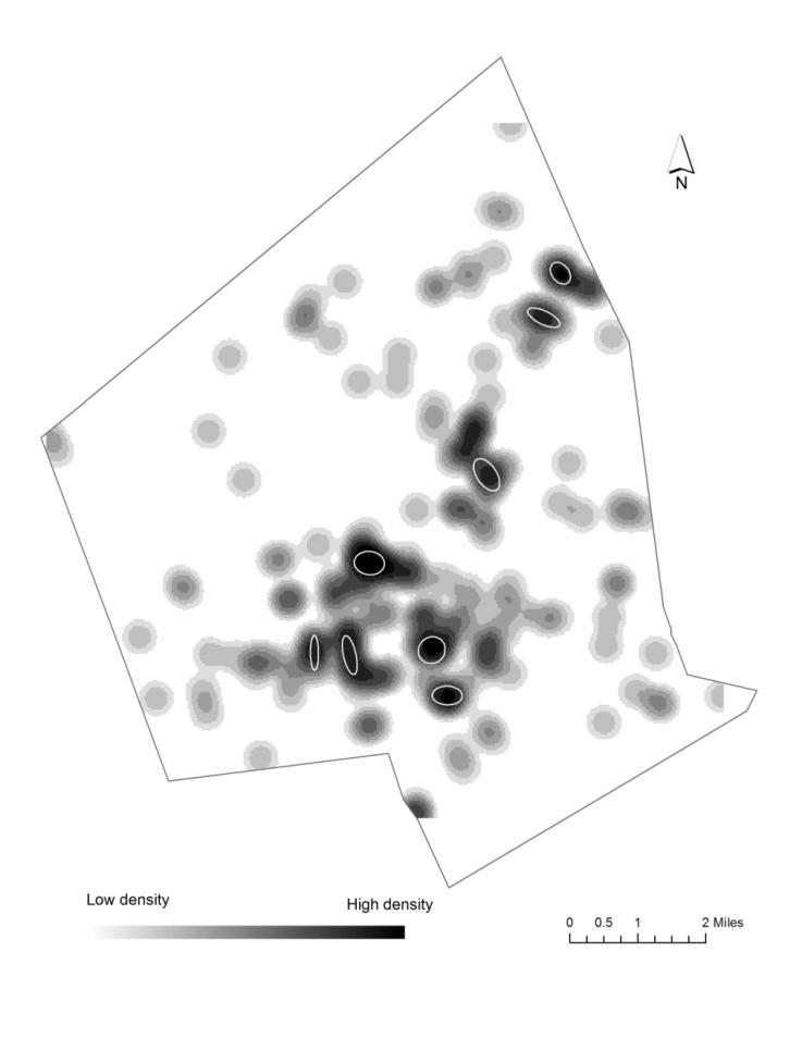
The study uses geographic information science (GIS) and statistics to find out if there are statistical differences between full term and preterm births to non-Hispanic white, non-Hispanic Black, and Hispanic mothers in their exposure to air pollution and access to environmental amenities (green space and vendors of healthy food) in the second largest city in New England, Worcester, Massachusetts. Proximity to a Toxic Release Inventory site has a statistically significant effect on preterm birth regardless of race. The air-pollution hazard score from the Risk Screening Environmental Indicators Model is also a statistically significant factor when preterm births are categorized into three groups based on the degree of prematurity. Proximity to green space and to a healthy food vendor did not have an effect on preterm births. The study also used cluster analysis and found statistically significant spatial clusters of high preterm birth volume for non-Hispanic white, non-Hispanic Black, and Hispanic mothers.
1.
Introduction
Elemental imbalances between producer and grazers can influence life-history traits such as growth, survival, and reproduction. Chemical contaminants can have similar impacts on these traits [5]. Recently, there have been experimental efforts to investigate any interactive effects of these stressors. Hansen et al. 2008 [8] found empirical evidence that Daphnia experience strong interactive effects of food quality and the contaminant fluoxetine on their survival, growth, and reproduction. Here they observed that Daphnia fed nutrient-rich algal food experience greater toxicity to fluoxetine. Ieromina et al. 2014 [11] observed that Daphnia fed nutrient-deficient algal food experience high toxicity to the contaminant imidacloprid. They also observed evidence that nutrient excess food can impact the reproductive output for D. magna. While Lessard et al. 2012 [13] observed no interactive effects between food nutrient content and an herbicide contaminant on Daphnia survival but observed great effects on Daphnia growth rates under nutrient-rich conditions.
The toxic contaminant mercury (Hg) can bioaccumulate in aquatic food chains as methylmercury (MeHg) posing a risk to ecosystems and humans [15]. Karimi et al. 2007 [12] shows stoichiometric constraints, such as food quality, can affect the accumulation of MeHg in Daphnia. The interactive effects of nutrient availability and aqueous Hg concentration may play a significant role in the bioaccumulation of MeHg. Recently, Peace et al. 2016 [20] developed a stoichiometric producer-grazer model subject to concurrent stoichiometric constraints and contaminant stressors. They parameterized the model for algae and Daphnia exposed to MeHg under variable phosphorus conditions. This model assumes the organisms pay an energy or carbon cost when exposed to contaminants, that reduce the growth rates based on a linear dose response of growth to concentrations of the toxicant.
Following the stoichiometric assumptions of the classical 14 model [14], the stoichiometric-toxicant model developed by Peace et al. 2016 [20] allows the producer Phosphorus:Carbon(P:C) ratio to vary while keeping the grazer P:C ratio constant. This assumption is based on the fact that, although grazer stoichiometries are variable, the range of variation is small compared to the range of producer stoichiometries [22]. This often results in elemental imbalances between grazers and their resources. The model assumes the producer is optimal food for the grazer if its P:C ratio is equal to or greater than the P:C of the grazer, thus incorporating the effects of low-nutrient food content on grazer dynamics.
However, it has been reported that grazer dynamics are also affected by excess food nutrient content [3,6]. This phenomenon, called the stoichiometric knife edge, reflects a reduction in animal growth not only by food with low Phosphorus(P) content but also by food with excessively high P content. Peace et al. 2013 [18] extended the 14 model [14] in order to incorporate the effects of excess nutrient food content on grazer's growth in the absence of toxicants. They did this by stoichiometrically modifying the grazer's ingestion rate and conversion efficiency. The model assumes the mechanism behind this stoichiometric knife edge phenomenon is the grazer's feeding behavior. It assumes that high P content of food causes the animal to strongly decrease their ingestion rate, perhaps leading to insufficient Carbon(C) intake and thus decreased growth rate. This extended model captures the consequences of imbalances from both low P:C and high P:C food resources in the absence of toxicants.
Peace et al. 2016 [20] investigate grazer growth dynamics exposed to a contaminant stresses while under nutrient limited conditions. However, this model does not incorporate the consequences of nutrient excess conditions. Here, we integrate the stoichiometric tox-mediated producer-grazer model [20] with the non-toxicant stoichiometric knife edge model [18]. This result is the first model that incorporates the impact of excess nutrients on the producer-grazer dynamics when subject to a toxicant. We parameterize the model for algae and Daphnina exposed to the toxicant MeHg and investigate the impact of varying P and light conditions.
2.
Model Formulation
We start with the Stoichiometric Toxicant-mediated predator-prey model developed by Peace et al 2016 [20] based on Huang et al. 2014 [10]:
where
variables $x$ and $y$ are the prey and predator population densities (mg C/L) respectively and $u$ and $v$ give the toxicant body burden, or the concentration of the toxicant in the prey and predator, respectively. The function $f(x)$ is the predator ingestion rate. By following the recommendation of the committee on toxicology of the National Research Council in 1992 and tested in Miller et al. 2000 [16], we use the power law to represent the relationship between toxicant concentrations and predator mortality rate. Predator mortality rate as a function of $v$, takes the form $d_2(v) = h_2v^I+m_2$ where $h_2$ and $I$ are positive constants for coefficient and exponent of the power function and $m_2$ is the natural loss rate, including both natural mortality and respiration. Parameter $\alpha_1$ is the prey maximal growth rate and $\alpha_2$ is the toxicant effect on prey reproduction. Parameters $a_1$ and $a_2$ are toxicant uptake rates and $\sigma_1$ and $\sigma_2$ are toxicant efflux rates for the prey and predator, respectively. Parameter $\beta_1$ where $0<\beta_1<1$ is the growth efficiency of the prey, $\beta_2$ is the toxicant effect on predator reproduction and $\xi$ is the predator toxicant assimilation efficiency. $T$ is the total toxicant in the system, $P$ is the total amount of phosphorus in the system and $\theta$ is the constant predator $P:C$ ratio.
The growth rates of both organisms are influenced by the respective body burdens. Toxicological constraints appear as maximum functions in the above Model (2.1). The maximum term $0\leq \max(0, 1-\alpha_2u)\leq 1$ comes from a linear dose-response for the gain rate of prey. Similarly, the term $\max(0, 1-\beta_2v)$ represents a linear dose-response for the predator growth efficiency. Population growth dynamics are also influence by nutrient availability. Stoichiometric constraints appear as minimum functions in the above Model (2.1). The minimum function $\min \left\{K, \frac{P-\theta y}{q} \right\}$ is used to describe the prey carrying capacity. The first input, $K$ is the prey carrying capacity in-terms of carbon or light availability. The second input $\frac{P-\theta y}{q}$ is the carrying capacity determined by phosphorus availability. The numerator here, $P-\theta y$, is the total amount of P available for the prey. This is based on the assumption that all P is either in the prey or the predator. The model assumes prey are extremely efficient at taking up nutrients and does not allow free nutrients to be dissolved in the environment. The consumer growth rate is is described by another minimum function, $\min\left(\beta_1, \frac{Q}{\theta}\right)$. The first input, $\beta_1$ is used when consumer growth is limited by carbon, the second input, $\frac{Q}{\theta}$ is used when consumer growth is limited by phosphorus.
In, Peace et al. 2016 [20] they incorporate stoichiometric nutrient limitation to the toxicant mediated predator prey model developed by Huang et al. 2014 [10]. The current models do not consider the effects of excess nutrient conditions. Here, we develop and analyze the first model that incorporates the impact of excess nutrients on predator-prey dynamics when subject to a toxicant.
The grazer's ingestion rate, $f(x)$ is a monotonic increasing and differentiable function, $f'(x)\ge 0, f(0) = 0 $. $f(x)$ is saturating with $\lim\limits_{x\rightarrow\infty}f(x) = c$. We assume the ingestion rate is a Holling type Ⅱ function of the form $f(x) = \frac{cx}{a+x}$ where, c is the maximal grazer's ingestion rate and a is the half saturation constant. By following Peace et al. 2013 [18] we assume that the grazer ingests $P$ up to the rate required for its maximal growth but not more. This assumption is based on empirical data from Plath and Boersma 2001[21] which leads to a new expression for the grazer ingestion rate. The ingestion rate, $f(x)$ is replaced by
The grazer's growth rate, $g(x, y) = \min\left\{\beta_1, \frac{Q}{\theta}\right\}u(x, y)$, can be written as
Since, $\beta_1f(x)<c$, we see that
This expression is also incorporated into the body burden equation and our system takes the following form:
2.1. Model Reduction
We parameterize our toxicant-mediated stoichiometric knife edged producer-grazer Model (2.3) to a system of algal (producer) and Daphinia (grazer), in order to investigate the effects of co-occurring phosphorus constraints and MeHg stressors on population dynamics and MeHg bioaccumulation. All parameter values were used in Peace et al. 2016 [20] and are listed in Table 1. For the following analysis we assume $I = 1$ for mathematical convenience. We non-dimensionalize system (2.3) to facilitate the mathematical analysis and rescale the model with the following non-dimensional parameters:
Dropping the tildes for simplicity, the dimensionless form of system (2.3) yields
According to the parameterization in Table 1, $\epsilon = 0.0576$. Since $\epsilon$ is sufficiently small the dynamics of the body burdens $u$ and $v$ are on a much faster time scale than the population dynamics of $x$ and $y$. Therefore we let $\epsilon\to0$ and apply a quasi-steady-state reduction in order to reduce the model to the slow subsystem. Applying this quasi-steady-state reduction and letting $\epsilon\to0$ yields
Now, substituting (2.6) and $Q = \frac{P-\theta y}{x}$ into (2.5a) and (2.5b) gives us the following quasi-steady-state non-dimensional system
3.
Model Analysis
Note that if $T>\sigma_1^2$ then the toxicant levels are too high for the prey to reproduce and grow and $(x, y)\to (0, 0)$. For the following analysis we assume that $T<\sigma_1^2$ and let $\mathbf{k} = \min\left\{K, \frac{P}{q}\right\}$.
Theorem 3.1. Solution of the system (2.7) with the initial conditions in the set
will remain there for all forward time.
Proof. First we show the solutions remain in the rectangle $\mathbf{R}$ defined by $\big[0, \mathbf{k}\big]\times\big[0, \frac{P}{\theta}\big]$, then we show solutions are also bounded by the inequality $qx+\theta y<P$. Let $S(t) = (x(t), y(t))$ be a solution of System (2.7) with $S(0) \in \mathbf R$. Assume there exists a time $t_1>0$ such that $S(t_1)$ touches or crosses a boundary of $\mathbf R$ for the first time. The following cases prove solutions remain in $\mathbf R$ by contradiction. Case 1 left boundary: $x(t_1) = 0$
Let $\overline{y} = \underset{t\in[0, t_1]}\max y(t) <\frac{P}{\theta}$. Then for every $t\in [0, t_1]$,
This implies that $x(t_1)\geq x(0)e^{\alpha t_1} > 0$, where $\alpha$ is a constant. This contradicts $x(t_1) = 0$ and proves that $S(t_1)$ does not reach this boundary.
Case 2 right boundary: $x(t_1) = \mathbf{k} = \min \left\{ K, \frac{P}{q}\right\}$
Then for every $t\in [0, t_1]$,
Then $x(t)<\mathbf{k}$ by a standard comparison argument. This contradicts $x(t_1) = \mathbf{k}$ and proves that the trajectory does not cross this boundary.
Case 3 bottom boundary : $y(t_1) = 0$
Then for every $t\in [0, t_1]$,
This implies that $y(t_1)\geq y(0)e^{\alpha t_1} > 0$, where $\alpha$ is a constant. This contradicts $y(t_1) = 0$ and proves that $S(t_1)$ does not reach this boundary.
Case 4 top boundary: $y(t_1) = \frac{P}{\theta}$
Then for every $t\in [0, t_1]$,
Then $y(t)<\frac{P}{\theta}$ by a standard comparison argument. This contradicts $y(t_1) = \frac{P}{\theta}$ and proves that the trajectory does not cross this boundary. The above cases prove the trajectories are bounded in $\mathbf{R}$. Now assume $S(0) \in \Omega$ and there exists a time $t_1>0$ such that $S(t_1)$ touches or crosses a boundary of $\Omega$ for the first time. The final case proves solutions remain in $\Omega$ by contradiction.
Case 5: $qx(t_1)+\theta y(t_1) = P$
Then $qx(t)+\theta y(t)<P$ for every $t\in [0, t_1)$ and $qx'(t)+\theta y'(t)\geq 0$
and
Then
a contradiction.
To investigate the equilibria we first rewrite system (2.7) in the following form
where,
The Jacobian takes the following forms
3.1. Boundary Equilibria
We investigate the equilibria
The local stability of $E_0 = (0, 0)$ is determined by the Jacobian in the following form,
Jacobian, $J(E_0)$ has the eigenvalues with opposite signs, thus $E_0$ is saddle point. In the absence of grazer, the carrying capacity of the producer depends only on the light and phosphorus availability, which we denote as
So, $x^* = \mathbf{k}$. The local stability of $E_1 = (\mathbf{k}, 0)$ is determined by the Jacobian in the following form,
The stability of $E_1(\mathbf{k}, 0)$ depends on the sign of $G(\mathbf{k}, 0)$. $E_1$ is locally asymptotically stable if $G(\mathbf{k}, 0)<0$ and $E_1$ is saddle point if $G(\mathbf{k}, 0)>0$.
3.2. Interior Euilibria
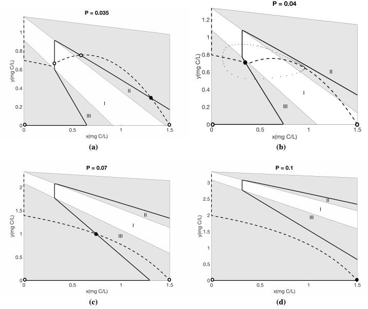
In this subsection, we analyze the existence and stability of the interior equilibrium numerically with phase plane analysis, Figure 1. The solution of the system are bounded by the trapezoidal region shown below. The phase plane is divided into three biologically significant regions by the two lines $\beta_1 = \frac{Q}{\theta}$ and $f(x) = \frac{c\theta}{Q}$. Region I is defined by $\beta_1<\frac{Q}{\theta}$ and $f(x)<\frac{c\theta}{Q}$. This represent the case where P is neither limiting nor in excess. Region Ⅱ is defined by $\beta_1>\frac{Q}{\theta}$; here, growth is limited by the deficiency of P. Region Ⅲ is defined by $\beta_1<\frac{Q}{\theta}$ and $f(x)>\frac{c\theta}{Q}$, where P is in excess and reduces grazer growth rate. Note that these same regions are described in Peace et al. 2013 [18] in the absence of toxicants.
4.
Numerical Analysis
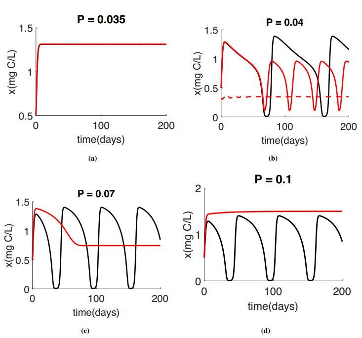
Peace et al. 2016 [20] investigate the effect of toxicant under stoichiometric constraints on the population dynamics for different light level. In this section we are comparing our result with [20]. We use the non-dimensionalized system of both models for simulations. The Black color will represent the results of Peace et al. 2016 [20] and the red color will represent our proposed model. Some instances the models agree and the red line is pllotted on top of the black line. These simulations use the parameter listed in Table 1 with K = 1.5mg C/L for varying Phosphorus level. All simulations used the Holling type Ⅱ function $f(x) = \frac{cx}{a+x}$ for the ingestion rate.
4.1. Numerical Simulations
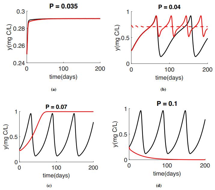
Numerical simulations of the reduced model, System (2.7) are presented for the producer in Figure 2 and the grazer in Figure 3 for varying values of P. The red simulations presented in figures 2 and 3 correspond to the phase planes presented in Figure 1.
For low P values we got the similar results as Peace et al. 2016 [20], see figures 2(a) and 3(a). As P increases, we start to see the differences between these two models. Figures 2(b) and 3(b) show the bistability for our proposed model, with a stable equilibria and a stable limit cycle. Under these same conditions, the populations oscillate for the Peace et al. 2016 [20] model. As we continue to increase P, the Peace et al. 2016 [20] model predicts similar oscillatory dynamics for moderate and high P values, however in the proposed model System (2.7), the oscillations collapse for higher P values, Figures 2(c, d) and 3(c, d). Very large values of P causes the extinction of grazer population, Figure 3(d).
4.2. Bifurcation Analysis
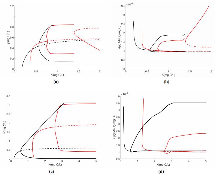
Here we perform a bifurcation analysis of the full model, System (2.3) using $K$ mg C/L as the bifurcation parameter for both low and high $P$ mg P/L, see Figure 4.
Qualitatively, the bifurcation diagrams for low P (Figures 4ab) and high P (Figures 4cd) are similar for both models. For low light levels, the grazer is at a stable equilibrium of a low density. As K increases this interior equilibrium loses stability and stable limit cycles emerge at a Hopf bifurcation. The limit cycles start off with small amplitudes, but as K continues to increase the amplitudes get bigger. Eventually for higher levels of K these limit cycles collapse and another interior equilibrium point gains stability. This occurs at a saddle node bifurcation. As K increases further to very high values the grazer density begins to decrease. Here, the grazer is limited by food quality, or P-limitation.
Under low P conditions we see differences between the two models for low K conditions (Figures 4ab). First, under very low K, there is region where the previous model predicts a stable grazer population at a low density, whereas our model predicts grazer extinction (Figure 4a). Under low light conditions Q, the algae P:C ratio, is large. In both models, there is a low quantity of food available for the grazers. In the previous model, the grazer is limited by food quantity. However, our model incorporates consequences of high P content, and the grazer is limited by food quality, This is the influence of the stoichiometric knife edge. It is important to note the differences in the predicted grazer body burdens at low K levels (Figure 4b). Here, there is range of low K values, where the previous models predicts lower body burdens than our model. We also observe a shift in the location of the Hopf bifurcation and the amplitude of the cycles. The previous model exhibits limit cycles at a lower value of light than our model, and the cycles have larger amplitude. For high light levels, the two models predict qualitatively similar dynamics. Indeed, here the low P and high K conditions yield low Q values. Here the grazer is limited by P in both models.
The differences between the predictions of the model are more significant under high P levels, where effects of the stoichiometric knife edge are more likely to be occur (Figures 4cd). Here, the entire bifurcation diagram is shift significantly to the right for our model, note the bifurcation diagram takes $K$ from 0 to 5 mg C/L, in these figures. Light levels above 5 mg C/L are unrealistic in natural and laboratory settings. The Hopf bifurcation occurs at much higher light levels. Consequently, the dynamics of the two models are qualitatively different even for high light levels.
5.
Conclusion
Elemental mismatches between trophic levels often leads to consequences on population growth. Food resources are rarely optimally suited for grazers in terms of their nutrient content. Daphnia grazers are often faced with P limitation, when their diet consists of algae with low P:C [22]. On the other hand, when their diet consists of algae with high P:C they have to deal with this P excess and can become limited by C [21,18,19]. These types of nutritional constraints influence life-history traits, such as growth rates and conversion efficiencies. Toxicants can have similar impacts on these life-history traits. We developed and analyzed the first model that incorporates the impact of both low and excess nutrients on the producer-grazer dynamics when subject to a toxicant. Previous models that consider concurrent nutrient and toxicological constraints consider only nutrient limited conditions [20]. Here, we expanded the model by Peace et al. 2016 [20] to incorporate the effects of nutrient excess conditions on population dynamics, a phenomenon called the stoichiometric knife edge. Peace et al. 2013 [18] modeled this phenomenon without the presence of toxicants. The proposed model (2.3) yields additional insights for risk assessment compared to previous work, especially under excess food nutrient conditions.
To facilitate the analysis of the model we assumed population metabolism occurs on a faster time scale than population growth dynamics. Considering the fast and slow systems in the model and a quasi-steady-state assumption we were able to reduce system (2.3) down to the two dimensional system (2.7). We showed the boundedness of the reduced system (2.7) analytically. We investigated the existence and local stability of boundary equilibria analytically. We numerically observed the existence and stability of interior equilibria and limit cycles.
We compared the proposed model (2.7) results with those of system (2.1) developed by Peace et al. 2016 [20]. For low values of P the population dynamics are similar (Figure 2a, Figure 3a), however they begin to deviate for moderate and high P loads (Figure 2b-d, Figure 3b-d). The Peace et al. 2016 [20] model predicts periodic cycles for moderate and high P loads, however our models captures the effects of excess P content on the populations and predicts extinction of the grazer population for high P value. The most important differences between the two model predictions can be seen in the bifurcation diagrams (Figure 4). In particular see Figure 4(b, d), under low light levels $K$ near 0.5 mg C/L our model predicts a high body burden for the grazer. Under these conditions previous models may be under predicting the effects of toxicants which can have important implications on risk assessment protocols developed using these models.
In order to incorporate the stoichiometric knife edge phenomenon we following the assumption of Peace et al. 2013 [18] and considered a reduction in grazer ingestion rate under high P food conditions. However, the mechanisms underlying this phenomenon is likely more complicated than a simple reduction in foraging behaviors [7]. For example nutrient and carbon absorption rates of ingested food, gut passage time, and other metabolic processes such as respiration rates may play a role. It is possible that these processes are also influences in the presence of a toxicant. Additional experiments on metabolic rates under multiple constraints can help us modify the models presented here to consider these extensions.
While these models are parameterized for a system of Daphnia and algal under varying P and MeHg conditions, the models have broader applicability. Reduction in growth rates when exposed to high nutrient conditions has been observed for a variety of species [21,4,17]. At the same time many system experience exposure to a multitude of anthropogenic and natural toxicants [25]. Re-parameterization of these models can yield additional insight into other ecological producer-grazer systems subject to concurrent stoichiometric and toxicological constraints.
Acknowledgements
This material is based upon work supported by the NSF under Grant No 1615697
Conflict of interest
All authors declare no conflicts of interest in this paper.


 DownLoad: