Mean time to infection by small diffusing droplets containing SARS-CoV-2 during close social contacts

U. Dobramysl; C. Sieben; D. Holcman; U. Dobramysl; C. Sieben; D. Holcman

doi:10.3934/nhm.2024017

Networks and Heterogeneous Media

2024, Volume 19, Issue 1: 384-404. doi: 10.3934/nhm.2024017

Previous Article Next Article

Research article Special Issues

Mean time to infection by small diffusing droplets containing SARS-CoV-2 during close social contacts

1.
Peter Medawar Building for Pathogen Research, Nuffield Department of Medicine, University of Oxford, Oxford, UK
2.
Nanoscale Infection Biology Group, Helmholtz Centre for Infection Research, 38124 Braunschweig, Germany
3.
Group of data modeling and computational biology, IBENS-PSL Ecole Normale Superieure, Paris, France

Received: 16 May 2023 Revised: 18 December 2023 Accepted: 29 December 2023 Published: 04 April 2024

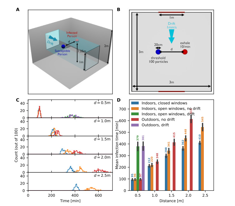
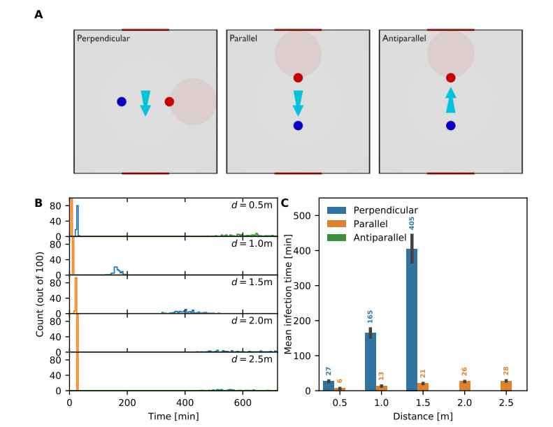
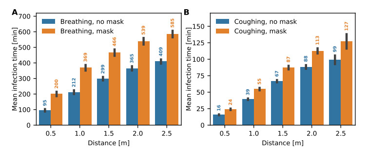
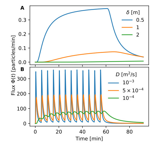
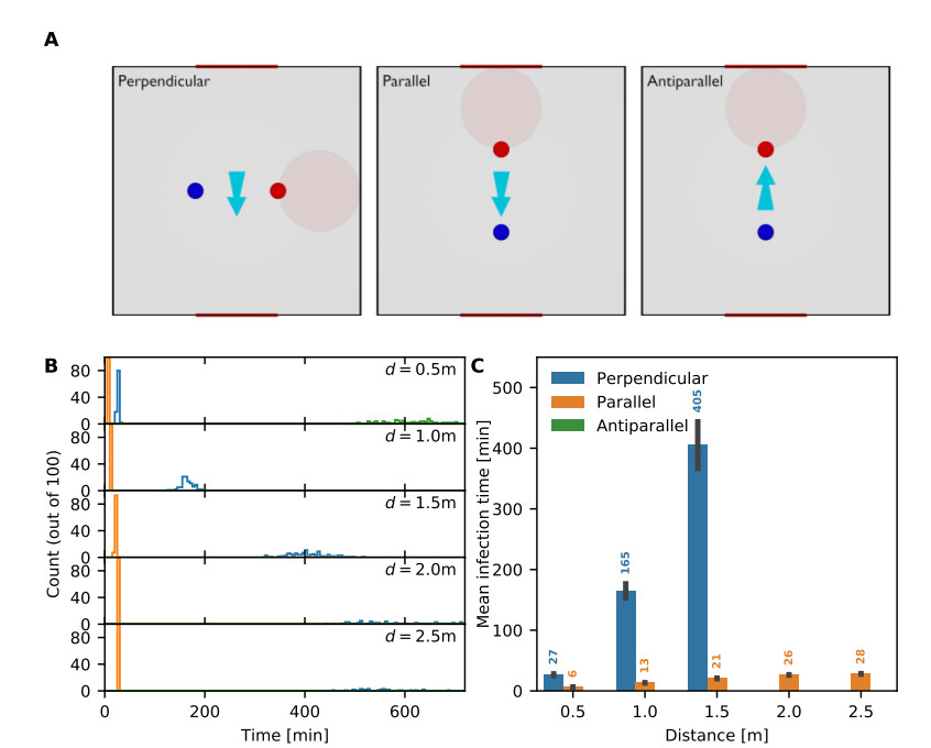
Airborne viruses such as SARS-CoV-2 are partly spread through aerosols containing viral particles. Inhalation of infectious airborne particles can lead to infection, a route that can be even more predominant than droplet or contact transmission. To study the transmission between a susceptible and an infected person, we estimated the distribution of arrival times of small diffusing aerosol particles to the inhaled region located below the nose until the number of particles reaches a critical threshold. Our results suggested that although contamination by continuous respiration can take approximately 90 min at a distance of 0.5 m, it is reduced to a few minutes when coughing or sneezing. Interestingly, there is not much difference between outdoors and indoors when the air is still. When a window is open inside an office, the infection time is reduced. Finally, wearing a mask leads to a delay in the time to infection. To conclude, diffusion analysis provides several key timescales of viral airborne transmission.
- aerosol diffusion,
- mean time to infection,
- simulations,
- modeling,
- SARS-CoV-2
Citation: U. Dobramysl, C. Sieben, D. Holcman. Mean time to infection by small diffusing droplets containing SARS-CoV-2 during close social contacts[J]. Networks and Heterogeneous Media, 2024, 19(1): 384-404. doi: 10.3934/nhm.2024017

Related Papers:

Abstract

Airborne viruses such as SARS-CoV-2 are partly spread through aerosols containing viral particles. Inhalation of infectious airborne particles can lead to infection, a route that can be even more predominant than droplet or contact transmission. To study the transmission between a susceptible and an infected person, we estimated the distribution of arrival times of small diffusing aerosol particles to the inhaled region located below the nose until the number of particles reaches a critical threshold. Our results suggested that although contamination by continuous respiration can take approximately 90 min at a distance of 0.5 m, it is reduced to a few minutes when coughing or sneezing. Interestingly, there is not much difference between outdoors and indoors when the air is still. When a window is open inside an office, the infection time is reduced. Finally, wearing a mask leads to a delay in the time to infection. To conclude, diffusion analysis provides several key timescales of viral airborne transmission.

References

[1]	R. H. Alford, J. A. Kasel, P. J. Gerone, V. Knight, Human influenza resulting from aerosol inhalation, Proceedings of the Society for Experimental Biology and Medicine, 122 (1966), 800–804. https://doi.org/10.3181/00379727-122-31255 doi: 10.3181/00379727-122-31255
[2]	M. Alsved, A. Matamis, R. Bohlin, M. Richter, P. E. Bengtsson, C. J. Fraenkel, et al., Exhaled respiratory particles during singing and talking, Aerosol Sci Tech, 54 (2020), 1245–1248. https://doi.org/10.1080/02786826.2020.1812502 doi: 10.1080/02786826.2020.1812502
[3]	P. Anfinrud, C. E. Bax, V. Stadnytskyi, A. Bax, Could Sars-Cov-2 be transmitted via speech droplets?, MedRxiv, [Preprint], (2020), [cited 2024 April 04]. Available from: https://doi.org/10.1101/2020.04.02.20051177
[4]	S. Asadi, A. S. Wexler, C. D. Cappa, S. Barreda, N. M. Bouvier, W. D. Ristenpart, Aerosol emission and superemission during human speech increase with voice loudness, Sci. Rep., 9 (2019), 1–10. https://doi.org/10.1038/s41598-019-38808-z doi: 10.1038/s41598-019-38808-z
[5]	M. P. Atkinson, L. M. Wein, Quantifying the routes of transmission for pandemic influenza, Bull. Math. Biol., 70 (2008), 820–867. https://doi.org/10.1007/s11538-007-9281-2 doi: 10.1007/s11538-007-9281-2
[6]	D. K. Chu, E. A. Akl, S. Duda, K. Solo, S. Yaacoub, H. J. Schünemann, et al., Physical distancing, face masks, and eye protection to prevent person-to-person transmission of Sars-Cov-2 and Covid-19: a systematic review and meta-analysis, The Lancet, 395 (2020), 1973–1987. https://doi.org/10.1016/S0140-6736(20)31142-9 doi: 10.1016/S0140-6736(20)31142-9
[7]	B. J. Cowling, D. K. Ip, V. J. Fang, P. Suntarattiwong, S. J. Olsen, J. Levy, et al., Aerosol transmission is an important mode of influenza a virus spread, Nat Commun, 4 (2013), 1–6. https://doi.org/10.1038/ncomms2922 doi: 10.1038/ncomms2922
[8]	EMG (Environmental and Modelling Group), Transmission of SARS-CoV-2 and Mitigating Measures. Scientific Advisory Group for Emergencies, 2020. Available from: https://www.gov.uk/government/publications/transmission-of-sars-cov-2-and-mitigating-measures-update-4-june-2020
[9]	P. Fabian, J. J. McDevitt, W. H. DeHaan, R. O. P. Fung, B. J. Cowling, K. H. Chan, et al., Influenza virus in human exhaled breath: An observational study, Plos One, 3 (2008), 1–6. https://doi.org/10.1371/journal.pone.0002691 doi: 10.1371/journal.pone.0002691
[10]	J. Gawn, M. Clayton, C. Makison, B. Crook, Evaluating the protection afforded by surgical masks against influenza bioaerosols, Health and Safety Executive, 2008. https://api.semanticscholar.org/CorpusID: 36385715
[11]	F. K. Gregson, N. A. Watson, C. M. Orton, A. E. Haddrell, L. P. McCarthy, T. J. Finnie, et al., Comparing aerosol concentrations and particle size distributions generated by singing, speaking and breathing, Aerosol Sci Tech, 55 (2021), 681–691. https://doi.org/10.1080/02786826.2021.1883544 doi: 10.1080/02786826.2021.1883544
[12]	K. M. Gustin, J. M. Katz, T. M. Tumpey, T. R. Maines, Comparison of the levels of infectious virus in respirable aerosols exhaled by ferrets infected with influenza viruses exhibiting diverse transmissibility phenotypes, J. Virol., 87 (2013), 7864–7873. https://doi.org/10.1128/jvi.00719-13 doi: 10.1128/jvi.00719-13
[13]	N. H. Leung, D. K. Chu, E. Y. Shiu, K. H. Chan, J. J. McDevitt, B. J. Hau, et al., Respiratory virus shedding in exhaled breath and efficacy of face masks, Nat. Med., 26 (2020), 676–680. https://doi.org/10.1038/s41591-020-0843-2 doi: 10.1038/s41591-020-0843-2
[14]	Q. Li, X. Guan, P. Wu, X. Wang, L. Zhou, Y. Tong, et al., Early transmission dynamics in wuhan, china, of novel coronavirus–infected pneumonia, N Engl J Med, 382 (2020), 1199–1207. https://doi/full/10.1056/NEJMOa2001316 doi: 10.1056/NEJMOa2001316
[15]	W. G. Lindsley, F. M. Blachere, K. A. Davis, T. A. Pearce, M. A. Fisher, R. Khakoo, et al., Distribution of airborne influenza virus and respiratory syncytial virus in an urgent care medical clinic, Clin. Infect. Dis., 50 (2010), 693–698. https://doi.org/10.1086/650457 doi: 10.1086/650457
[16]	W. G. Lindsley, T. A. Pearce, J. B. Hudnall, K. A. Davis, S. M. Davis, M. A. Fisher, et al., Quantity and size distribution of cough-generated aerosol particles produced by influenza patients during and after illness, J Occup Environ Hyg, 9 (2012), 443–449. https://doi.org/10.1080/15459624.2012.684582 doi: 10.1080/15459624.2012.684582
[17]	Y. Liu, Z. Ning, Y. Chen, M. Guo, Y. Liu, N. K. Gali, et al., Aerodynamic analysis of Sars-Cov-2 in two wuhan hospitals, Nature, 582 (2020), 557–560. https://doi.org/10.1038/s41586-020-2271-3 doi: 10.1038/s41586-020-2271-3
[18]	D. K. Milton, M. P. Fabian, B. J. Cowling, M. L. Grantham, J. J. McDevitt, Influenza virus aerosols in human exhaled breath: particle size, culturability, and effect of surgical masks, Plos Pathog, 9 (2013), e1003205. https://doi.org/10.1371/journal.ppat.1003205 doi: 10.1371/journal.ppat.1003205
[19]	N. Nikitin, E. Petrova, E. Trifonova, O. Karpova, Influenza virus aerosols in the air and their infectiousness, Adv. Virus. Res., 2014. https://doi.org/10.1155/2014/859090 doi: 10.1155/2014/859090
[20]	H. Qian, T. Miao, L. Li, X. Zheng, D. Luo, Y. Li, Indoor transmission of Sars-Cov-2, Indoor Air, 31 (2020), 639–645. https://doi.org/10.1111/ina.12766 doi: 10.1111/ina.12766
[21]	J. Reingruber, A. Papale, D. Holcman, Monitoring and predicting Sars-Cov-2 epidemic in france after deconfinement using a multiscale and age-dependent model, MedRxiv, [Preprint], (2020), [cited 2024 April 04]. Available from: https://doi.org/10.1101/2020.05.15.20099465
[22]	Roundups and Rapid Reactions, Expert reaction to questions about covid-19 and viral load. Science Media Centre, 2020. Available from https://www.sciencemediacentre.org/expert-reaction-to-questions-about-covid-19-and-viral-load.
[23]	S. Samuel, Why you're unlikely to get the coronavirus from runners or cyclists, VOX, 2020. Available from: https://www.vox.com/future-perfect/2020/4/24/21233226/coronavirus-runners-cyclists-airborne-infectious-dose
[24]	Z. Schuss, Theory and applications of stochastic processes: an analytical approach, Berlin: Springer Science & Business Media, 2009.
[25]	J. H. Seinfeld, S. N. Pandis, Atmospheric chemistry and physics: from air pollution to climate change, New York: John Wiley & Sons, 2016.
[26]	V. Stadnytskyi, C. E. Bax, A. Bax, P. Anfinrud, The airborne lifetime of small speech droplets and their potential importance in Sars-Cov-2 transmission, PNAS, 117 (2020), 11875–11877. https://doi.org/10.1073/pnas.2006874117 doi: 10.1073/pnas.2006874117
[27]	J. W. Tang, W. P. Bahnfleth, P. M. Bluyssen, G. Buonanno, J. L. Jimenez, J. Kurnitski, et al., Dismantling myths on the airborne transmission of severe acute respiratory syndrome coronavirus-2 (Sars-Cov-2), J. Hosp. Infect., 110 (2021), 89–96. https://doi.org/10.1016/j.jhin.2020.12.022 doi: 10.1016/j.jhin.2020.12.022
[28]	R. Tellier, Review of aerosol transmission of influenza a virus, Emerg Infect Dis., 12 (2006), 1657–1662. https://doi.org/10.3201%2Feid1211.060426
[29]	R. Tellier, Aerosol transmission of influenza a virus: a review of new studies, J. R. Soc. Interface., 6 (2009), S783–S790. https://doi.org/10.1098/rsif.2009.0302.focus doi: 10.1098/rsif.2009.0302.focus
[30]	R. Tellier, Y. Li, B. J. Cowling, J. W. Tang, Recognition of aerosol transmission of infectious agents: a commentary, BMC Infect Dis, 19 (2019), 1–9. https://doi.org/10.1186/s12879-019-3707-y doi: 10.1186/s12879-019-3707-y
[31]	J. Wang, G. Du, Covid-19 may transmit through aerosol, Ir J Med Sci, 189 (2020), 1143–1144. https://doi.org/10.1007/s11845-020-02218-2 doi: 10.1007/s11845-020-02218-2
[32]	C. Ward, M. Dempsey, C. Ring, R. Kempson, L. Zhang, D. Gor, et al., Design and performance testing of quantitative real time pcr assays for influenza a and b viral load measurement, J Clin Virol, 29 (2004), 179–188. https://doi.org/10.1016/S1386-6532(03)00122-7 doi: 10.1016/S1386-6532(03)00122-7
[33]	J. Yan, M. Grantham, J. Pantelic, P. J. B. De Mesquita, B. Albert, F. Liu, et al., Infectious virus in exhaled breath of symptomatic seasonal influenza cases from a college community, PNAS, 115 (2018), 1081–1086. https://doi.org/10.1073/pnas.1716561115 doi: 10.1073/pnas.1716561115

Reader Comments

Your name:*

Email:*
© 2024 the Author(s), licensee AIMS Press. This is an open access article distributed under the terms of the Creative Commons Attribution License (http://creativecommons.org/licenses/by/4.0)