Simple is best: A single-CNN method for classifying remote sensing images

Huaxiang Song; Yong Zhou; Huaxiang Song; Yong Zhou

doi:10.3934/nhm.2023070

Networks and Heterogeneous Media

2023, Volume 18, Issue 4: 1600-1629. doi: 10.3934/nhm.2023070

Previous Article Next Article

Research article

Simple is best: A single-CNN method for classifying remote sensing images

Huaxiang Song ^,,
Yong Zhou

School of Geography Science and Tourism, Hunan University of Arts and Science, Changde, China

Received: 18 June 2023 Revised: 13 August 2023 Accepted: 22 August 2023 Published: 05 September 2023

Recently, researchers have proposed a lot of methods to boost the performance of convolutional neural networks (CNNs) for classifying remote sensing images (RSI). However, the methods' performance improvements were insignificant, while time and hardware costs increased dramatically due to re-modeling. To tackle this problem, this study sought a simple, lightweight, yet more accurate solution for RSI semantic classification (RSI-SC). At first, we proposed a set of mathematical derivations to analyze and identify the best way among different technical roadmaps. Afterward, we selected a simple route that can significantly boost a single CNN's performance while maintaining simplicity and reducing costs in time and hardware. The proposed method, called RE-EfficientNet, only consists of a lightweight EfficientNet-B3 and a concise training algorithm named RE-CNN. The novelty of RE-EfficientNet and RE-CNN includes the following: First, EfficientNet-B3 employs transfer learning from ImageNet-1K and excludes any complicated re-modeling. It can adequately utilize the easily accessible pre-trained weights for time savings and avoid the pre-training effect being weakened due to re-modeling. Second, RE-CNN includes an effective combination of data augmentation (DA) transformations and two modified training tricks (TTs). It can alleviate the data distribution shift from DA-processed training sets and make the TTs more effective through modification according to the inherent nature of RSI. Extensive experimental results on two RSI sets prove that RE-EfficientNet can surpass all 30 cutting-edge methods published before 2023. It gives a remarkable improvement of 0.50% to 0.75% in overall accuracy (OA) and a 75% or more reduction in parameters. The ablation experiment also reveals that RE-CNN can improve CNN OA by 0.55% to 1.10%. All the results indicate that RE-EfficientNet is a simple, lightweight and more accurate solution for RSI-SC. In addition, we argue that the ideas proposed in this work about how to choose an appropriate model and training algorithm can help us find more efficient approaches in the future.
- RE-EfficientNet,
- RE-CNN,
- remote sensing image classification,
- deep learning
Citation: Huaxiang Song, Yong Zhou. Simple is best: A single-CNN method for classifying remote sensing images[J]. Networks and Heterogeneous Media, 2023, 18(4): 1600-1629. doi: 10.3934/nhm.2023070

Related Papers:

Abstract

Recently, researchers have proposed a lot of methods to boost the performance of convolutional neural networks (CNNs) for classifying remote sensing images (RSI). However, the methods' performance improvements were insignificant, while time and hardware costs increased dramatically due to re-modeling. To tackle this problem, this study sought a simple, lightweight, yet more accurate solution for RSI semantic classification (RSI-SC). At first, we proposed a set of mathematical derivations to analyze and identify the best way among different technical roadmaps. Afterward, we selected a simple route that can significantly boost a single CNN's performance while maintaining simplicity and reducing costs in time and hardware. The proposed method, called RE-EfficientNet, only consists of a lightweight EfficientNet-B3 and a concise training algorithm named RE-CNN. The novelty of RE-EfficientNet and RE-CNN includes the following: First, EfficientNet-B3 employs transfer learning from ImageNet-1K and excludes any complicated re-modeling. It can adequately utilize the easily accessible pre-trained weights for time savings and avoid the pre-training effect being weakened due to re-modeling. Second, RE-CNN includes an effective combination of data augmentation (DA) transformations and two modified training tricks (TTs). It can alleviate the data distribution shift from DA-processed training sets and make the TTs more effective through modification according to the inherent nature of RSI. Extensive experimental results on two RSI sets prove that RE-EfficientNet can surpass all 30 cutting-edge methods published before 2023. It gives a remarkable improvement of 0.50% to 0.75% in overall accuracy (OA) and a 75% or more reduction in parameters. The ablation experiment also reveals that RE-CNN can improve CNN OA by 0.55% to 1.10%. All the results indicate that RE-EfficientNet is a simple, lightweight and more accurate solution for RSI-SC. In addition, we argue that the ideas proposed in this work about how to choose an appropriate model and training algorithm can help us find more efficient approaches in the future.

References

[1]	A. P. Plageras, K. E. Psannis, C. Stergiou, H. Wang, B. B. Gupta, Efficient IoT-based sensor BIG Data collection–processing and analysis in smart buildings. Future Gener Comput Syst, 82 (2018), 349–357. https://doi.org/10.1016/j.future.2017.09.082 doi: 10.1016/j.future.2017.09.082
[2]	Z. Ahmed, M. Ayaz, M. A. Hijji, M. Z. Abbas, A. Rahim, AUV-Based efficient data collection scheme for underwater linear sensor networks. Int J Semant Web Inf Syst, 18 (2022), 1–19. https://doi.org/10.4018/IJSWIS.299858 doi: 10.4018/IJSWIS.299858
[3]	D. Tian, Y. Han, B. Wang, T. Guan, H. Gu, W. Wei, Review of object instance segmentation based on deep learning, J. Electron. Imag., 31 (2021), 041205. https://doi.org/10.1117/1.JEI.31.4.041205 doi: 10.1117/1.JEI.31.4.041205
[4]	K. S. Arikumar, A. D. Kumar, T. R. Gadekallu, S. B. Prathiba, K. Tamilarasi, Real-Time 3D Object detection and classification in autonomous driving environment using 3D LiDAR and camera sensors, Electronics, 11 (2022), 4203. https://doi.org/10.3390/electronics11244203 doi: 10.3390/electronics11244203
[5]	H. Song, A more efficient approach for remote sensing image classification, Comput. Mater. Contin., 74 (2023), 5741–5756. https://doi.org/10.32604/cmc.2023.034921 doi: 10.32604/cmc.2023.034921
[6]	H. Song, FST-EfficientNetV2: exceptional image classification for remote sensing, Comput. Sci. Eng., 46 (2023), 3959–3978. https://doi.org/10.32604/csse.2023.038429 doi: 10.32604/csse.2023.038429
[7]	H. Touvron, A. Vedaldi, M. Douze, H. Jégou, Fixing the train-test resolution discrepancy, arXiv: 1906.06423, [preprint], (2019)[cited 2023 September 05]. Available from: http://arXiv.org/abs/1906.06423
[8]	H. Song, A Leading but Simple Classification Method for Remote Sensing Images, AETiC, 7 (2023), 1–20. https://doi.org/10.33166/AETiC.2023.03.001 doi: 10.33166/AETiC.2023.03.001
[9]	M. Tan, Q. V. Le, EfficientNet: Rethinking Model Scaling for Convolutional Neural Networks, arXiv: 1905.11946, [preprint], (2019)[cited 2023 September 05]. Available from: http://arXiv.org/abs/1905.11946
[10]	G. Cheng, C. Yang, X. Yao, L. Guo, J. Han, When deep learning meets metric learning: remote sensing image scene classification via learning discriminative CNNs, IEEE Trans Geosci Remote Sens, 56 (2018), 2811–2821. https://doi.org/10.1109/TGRS.2017.2783902 doi: 10.1109/TGRS.2017.2783902
[11]	Y. Guo, J. Ji, X. Lu, H. Huo, T. Fang, D. Li, Global-Local attention network for aerial scene classification, IEEE Access, 7 (2019), 67200–67212. https://doi.org/10.1109/ACCESS.2019.2918732 doi: 10.1109/ACCESS.2019.2918732
[12]	R. Minetto, M. P. Segundo, S. Sarkar, Hydra: An ensemble of convolutional neural networks for geospatial land classification, IEEE Trans Geosci Remote Sens, 57 (2019), 6530–6541. https://doi.org/10.1109/TGRS.2019.2906883 doi: 10.1109/TGRS.2019.2906883
[13]	W. Tong, W. Chen, W. Han, X. Li, L. Wang, Channel-Attention-Based DenseNet network for remote sensing image scene classification, IEEE J Sel Top Appl Earth Obs Remote Sens, 13 (2020), 4121–4132. https://doi.org/10.1109/JSTARS.2020.3009352 doi: 10.1109/JSTARS.2020.3009352
[14]	J. Li, D. Lin, Y. Wang, G. Xu, C. Ding, Deep discriminative representation learning with attention map for scene classification, arXiv: 1902.07967, [preprint], (2019)[cited 2023 September 05]. Available from: http://arXiv.org/abs/1902.07967
[15]	H. Alhichri, A. S. Alswayed, Y. Bazi, N. Ammour, N. A. Alajlan, Classification of remote sensing images using efficientnet-b3 cnn model with attention, IEEE Access, 9 (2021), 14078–14094. https://doi.org/10.1109/ACCESS.2021.3051085 doi: 10.1109/ACCESS.2021.3051085
[16]	B. Li, Y. Guo, J. Yang, L. Wang, Y. Wang, W. An, Gated recurrent multiattention network for VHR remote sensing image classification, IEEE Trans Geosci Remote Sens, 60 (2022), 1–13. https://doi.org/10.1109/TGRS.2021.3093914 doi: 10.1109/TGRS.2021.3093914
[17]	W. Chen, S. Ouyang, W. Tong, X. Li, X. Zheng, L. Wang, GCSANet: A global context spatial attention deep learning network for remote sensing scene classification, IEEE J Sel Top Appl Earth Obs Remote Sens, 15 (2022), 1150–1162. https://doi.org/10.1109/JSTARS.2022.3141826 doi: 10.1109/JSTARS.2022.3141826
[18]	Q. Zhao, Y. Ma, S. Lyu, L. Chen, Embedded Self-Distillation in compact multibranch ensemble network for remote sensing scene classification, IEEE Trans Geosci Remote Sens, 60 (2022), 1–15. https://doi.org/10.1109/TGRS.2021.3126770 doi: 10.1109/TGRS.2021.3126770
[19]	H. Song, A consistent mistake in remote sensing images' classification literature, Intell. Autom. Soft Comput., 37 (2023), 1381–1398. https://doi.org/10.32604/iasc.2023.039315 doi: 10.32604/iasc.2023.039315
[20]	S. Chaib, H. Liu, Y. Gu, H. Yao, Deep feature fusion for vhr remote sensing scene classification, IEEE Trans Geosci Remote Sens, 55 (2017), 4775–4784. https://doi.org/10.1109/TGRS.2017.2700322 doi: 10.1109/TGRS.2017.2700322
[21]	Y. Liu, C. Y. Suen, Y. Liu, L. Ding, Scene classification using hierarchical wasserstein CNN, IEEE Trans Geosci Remote Sens, 57 (2019), 2494–2509. https://doi.org/10.1109/TGRS.2018.2873966 doi: 10.1109/TGRS.2018.2873966
[22]	Y. Liu, Y. Liu, L. Ding, Scene classification by coupling convolutional neural networks with wasserstein distance, IEEE Geosci. Remote Sensing Lett., 16 (2019), 722–726. https://doi.org/10.1109/LGRS.2018.2883310 doi: 10.1109/LGRS.2018.2883310
[23]	Y. Bazi, M. M. Al Rahhal, H. Alhichri, N. Alajlan, Simple yet effective fine-tuning of deep CNNs using an auxiliary classification loss for remote sensing scene classification, Remote Sensing, 11 (2019), 2908. https://doi.org/10.3390/rs11242908 doi: 10.3390/rs11242908
[24]	W. Zhang, P. Tang, L. Zhao, Remote sensing image scene classification using CNN-CapsNet, Remote Sensing, 11 (2019), 494. https://doi.org/10.3390/rs11050494 doi: 10.3390/rs11050494
[25]	J. Xie, N. He, L. Fang, A. Plaza, Scale-Free convolutional neural network for remote sensing scene classification, IEEE Trans Geosci Remote Sens, 57 (2019), 6916–6928. https://doi.org/10.1109/TGRS.2019.2909695 doi: 10.1109/TGRS.2019.2909695
[26]	H. Sun, S. Li, X. Zheng, X. Lu, Remote sensing scene classification by gated bidirectional network, IEEE Trans Geosci Remote Sens, 58 (2020), 82–96. https://doi.org/10.1109/TGRS.2019.2931801 doi: 10.1109/TGRS.2019.2931801
[27]	D. Guo, Y. Xia, X. Luo, Scene classification of remote sensing images based on saliency dual attention residual network, IEEE Access, 8 (2020), 6344–6357. https://doi.org/10.1109/ACCESS.2019.2963769 doi: 10.1109/ACCESS.2019.2963769
[28]	X. Tang, Q. Ma, X. Zhang, F. Liu, J. Ma, L. Jiao, Attention consistent network for remote sensing scene classification, IEEE J Sel Top Appl Earth Obs Remote Sens, 14 (2021), 2030–2045. https://doi.org/10.1109/JSTARS.2021.3051569 doi: 10.1109/JSTARS.2021.3051569
[29]	Y. Bazi, L. Bashmal, M. M. A. Rahhal, R. A. Dayil, N. A. Ajlan, Vision transformers for remote sensing image classification, Remote Sensing, 13 (2021), 516. https://doi.org/10.3390/rs13030516 doi: 10.3390/rs13030516
[30]	J. Zhang, H. Zhao, J. Li, TRS: transformers for remote sensing scene classification, Remote Sensing, 13 (2021), 4143. https://doi.org/10.3390/rs13204143 doi: 10.3390/rs13204143
[31]	D. Wang, J. Zhang, B. Du, G. S. Xia, D. Tao, An empirical study of remote sensing pretraining, arXiv: 2204.02825, [preprint], (2022)[cited 2023 September 06]. Available from: http://arXiv.org/abs/2204.02825
[32]	C. Shi, X. Zhang, J. Sun, L. Wang, Remote sensing scene image classification based on Self-Compensating convolution neural network, Remote Sensing, 14 (2022), 545. https://doi.org/10.3390/rs14030545 doi: 10.3390/rs14030545
[33]	S. B. Chen, Q. S. Wei, W. Z. Wang, J. Tang, B. Luo, Z. Y. Wang, Remote sensing scene classification via Multi-Branch local attention network, IEEE Trans. on Image Process., 31 (2022), 99–109. https://doi.org/10.1109/TIP.2021.3127851 doi: 10.1109/TIP.2021.3127851
[34]	P. Deng, K. Xu, H. Huang, When CNNs meet vision transformer: a joint framework for remote sensing scene classification, IEEE Geosci. Remote Sensing Lett., 19 (2022), 1–5. https://doi.org/10.1109/LGRS.2021.3109061 doi: 10.1109/LGRS.2021.3109061
[35]	W. Miao, J. Geng, W. Jiang, Multigranularity decoupling network with pseudolabel selection for remote sensing image scene classification, IEEE Trans Geosci Remote Sens, 61 (2023), 1–13. https://doi.org/10.1109/TGRS.2023.3244565 doi: 10.1109/TGRS.2023.3244565
[36]	H. Song, W. Yang, GSCCTL: a general semi-supervised scene classification method for remote sensing images based on clustering and transfer learning, Int J Remote Sens., 43 (2022), 5976–6000. https://doi.org/10.1080/01431161.2021.2019851 doi: 10.1080/01431161.2021.2019851
[37]	W. Wang, Y. Chen, P. Ghamisi, Transferring CNN with adaptive learning for remote sensing scene classification, IEEE Trans Geosci Remote Sens, 60 (2022), 1–18. https://doi.org/10.1109/TGRS.2022.3190934 doi: 10.1109/TGRS.2022.3190934
[38]	K. Xu, P. Deng, H. Huang, Vision transformer: an excellent teacher for guiding small networks in remote sensing image scene classification, IEEE Trans Geosci Remote Sens, 60 (2022), 1–15. https://doi.org/10.1109/TGRS.2022.3152566 doi: 10.1109/TGRS.2022.3152566
[39]	T. He, Z. Zhang, H. Zhang, Z. Zhang, J. Xie, M. Li, Bag of tricks for image classification with convolutional neural networks, Proceedings of the IEEE/CVF conference on computer vision and pattern recognition, (2019), 558–567.
[40]	S. Yun, D. Han, S. J. Oh, S. Chun, J. Choe, Y. Yoo, CutMix: Regularization strategy to train strong classifiers with localizable features, Proceedings of the IEEE/CVF international conference on computer vision, (2019), 6023–6032.
[41]	C. B. Zhang, P. T. Jiang, Q. Hou, Y. Wei, Q. Han, Z. Li, et al., Delving deep into label smoothing, IEEE Trans. on Image Process., 30 (2021), 5984–5996. https://doi.org/10.1109/TIP.2021.3089942 doi: 10.1109/TIP.2021.3089942
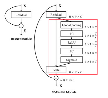
[42]	J. Hu, L. Shen, S. Albanie, G. Sun, E. Wu, Squeeze-and-Excitation Networks, Proceedings of the IEEE conference on computer vision and pattern recognition, (2018), 7132–7141.
[43]	R. R. Selvaraju, M. Cogswell, A. Das, R. Vedantam, D. Parikh, D. Batra, Grad-CAM: visual explanations from deep networks via Gradient-Based localization, Proceedings of the IEEE international conference on computer vision, (2017), 618–626.
[44]	I. Loshchilov, F. Hutter, Decoupled weight decay regularization, arXiv: 1711.05101v3, [preprint], (2017)[cited 2023 September 05]. Available from: http://arXiv.org/abs/1711.05101v3
[45]	C. Szegedy, V. Vanhoucke, S. Ioffe, J. Shlens, Z. Wojna, Rethinking the inception architecture for computer vision, Proceedings of the IEEE conference on computer vision and pattern recognition, 2016, 2818–2826.
[46]	H. Zhang, M. Cisse, Y. N. Dauphin, D. Lopez-Paz, Mixup: beyond empirical risk minimization, arXiv: 1710.09412, [preprint], (2017)[cited 2023 September 05]. Available from: http://arXiv.org/abs/1710.09412
[47]	Y. H. Liu, E. Sangineto, W. Bi, N. Sebe, B. Lepri, M. Nadai, Efficient training of visual transformers with small datasets, NIPS, 34 (2021), 23818–23830.
[48]	A. Hassani, S. Walton, N. Shah, A. Abuduweili, J. Li, H. Shi, Escaping the big data paradigm with compact transformers, arXiv: 2104.05704, [preprint], (2021)[cited 2023 September 05]. Available from: http://arXiv.org/abs/2104.05704
[49]	Z. Li, F. Liu, W. Yang, S. Peng, J. Zhou, A survey of convolutional neural networks: analysis, applications, and prospects, IEEE Trans. Neural Netw. Learning Syst., 33 (2022), 6999–7019. https://doi.org/10.1109/TNNLS.2021.3084827 doi: 10.1109/TNNLS.2021.3084827
[50]	F. Liu, D. Chen, Z. Guan, X. Zhou, J. Zhu, J. Zhou, RemoteCLIP: A vision language foundation model for remote sensing, arXiv: 2306.11029, [preprint], (2023)[cited 2023 September 05]. Available from: http://arXiv.org/abs/2306.11029
[51]	L van der Maaten, G. Hinton, Visualizing data using t-SNE, J Mach Learn Res, 9 (2008), 2579–2605.
[52]	Y. Long, G. S. Xia, S. Li, W. Yang, M. Y. Yang, X. X. Zhu, et al., On creating benchmark dataset for aerial image interpretation: reviews, guidances, and Million-AID, IEEE J Sel Top Appl Earth Obs Remote Sens, 14 (2021), 4205–4230. https://doi.org/10.1109/JSTARS.2021.3070368 doi: 10.1109/JSTARS.2021.3070368

Reader Comments

Your name:*

Email:*
© 2023 the Author(s), licensee AIMS Press. This is an open access article distributed under the terms of the Creative Commons Attribution License (http://creativecommons.org/licenses/by/4.0)