Controlled cellular automata

  • Received: 01 July 2018
  • Primary: 93C55, 92B05; Secondary: 93C95

  • Cellular Automata have been successfully used to model evolution of complex systems based on simples rules. In this paper we introduce controlled cellular automata to depict the dynamics of systems with controls that can affect their evolution. Using theory from discrete control systems, we derive results for the control of cellular automata in specific cases. The paper is mostly oriented toward two applications: fire spreading; morphogenesis and tumor growth. In both cases, we illustrate the impact of a control on the evolution of the system. For the fire, the control is assumed to be either firelines or firebreaks to prevent spreading or dumping of water, fire retardant and chemicals (foam) on the fire to neutralize it. In the case of cellular growth, the control describes mechanisms used to regulate growth factors and morphogenic events based on the existence of extracellular matrix structures called fractones. The hypothesis is that fractone distribution may coordinate the timing and location of neural cell proliferation, thereby guiding morphogenesis, at several stages of early brain development.

    Citation: Achilles Beros, Monique Chyba, Oleksandr Markovichenko. Controlled cellular automata[J]. Networks and Heterogeneous Media, 2019, 14(1): 1-22. doi: 10.3934/nhm.2019001
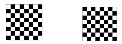
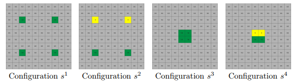
    Related Papers:

    [1] Achilles Beros, Monique Chyba, Oleksandr Markovichenko . Controlled cellular automata. Networks and Heterogeneous Media, 2019, 14(1): 1-22. doi: 10.3934/nhm.2019001
    [2] Fabio Della Rossa, Carlo D’Angelo, Alfio Quarteroni . A distributed model of traffic flows on extended regions. Networks and Heterogeneous Media, 2010, 5(3): 525-544. doi: 10.3934/nhm.2010.5.525
    [3] Richard Carney, Monique Chyba, Taylor Klotz . Using hybrid automata to model mitigation of global disease spread via travel restriction. Networks and Heterogeneous Media, 2024, 19(1): 324-354. doi: 10.3934/nhm.2024015
    [4] Ingenuin Gasser, Marcus Kraft . Modelling and simulation of fires in tunnel networks. Networks and Heterogeneous Media, 2008, 3(4): 691-707. doi: 10.3934/nhm.2008.3.691
    [5] Didier Georges . Infinite-dimensional nonlinear predictive control design for open-channel hydraulic systems. Networks and Heterogeneous Media, 2009, 4(2): 267-285. doi: 10.3934/nhm.2009.4.267
    [6] Mahmoud Saleh, Endre Kovács, Nagaraja Kallur . Adaptive step size controllers based on Runge-Kutta and linear-neighbor methods for solving the non-stationary heat conduction equation. Networks and Heterogeneous Media, 2023, 18(3): 1059-1082. doi: 10.3934/nhm.2023046
    [7] Marco Scianna, Luca Munaron . Multiscale model of tumor-derived capillary-like network formation. Networks and Heterogeneous Media, 2011, 6(4): 597-624. doi: 10.3934/nhm.2011.6.597
    [8] Anna Chiara Lai, Paola Loreti . Self-similar control systems and applications to zygodactyl bird's foot. Networks and Heterogeneous Media, 2015, 10(2): 401-419. doi: 10.3934/nhm.2015.10.401
    [9] Xavier Litrico, Vincent Fromion, Gérard Scorletti . Robust feedforward boundary control of hyperbolic conservation laws. Networks and Heterogeneous Media, 2007, 2(4): 717-731. doi: 10.3934/nhm.2007.2.717
    [10] Klaus-Jochen Engel, Marjeta Kramar FijavŽ . Exact and positive controllability of boundary control systems. Networks and Heterogeneous Media, 2017, 12(2): 319-337. doi: 10.3934/nhm.2017014
  • Cellular Automata have been successfully used to model evolution of complex systems based on simples rules. In this paper we introduce controlled cellular automata to depict the dynamics of systems with controls that can affect their evolution. Using theory from discrete control systems, we derive results for the control of cellular automata in specific cases. The paper is mostly oriented toward two applications: fire spreading; morphogenesis and tumor growth. In both cases, we illustrate the impact of a control on the evolution of the system. For the fire, the control is assumed to be either firelines or firebreaks to prevent spreading or dumping of water, fire retardant and chemicals (foam) on the fire to neutralize it. In the case of cellular growth, the control describes mechanisms used to regulate growth factors and morphogenic events based on the existence of extracellular matrix structures called fractones. The hypothesis is that fractone distribution may coordinate the timing and location of neural cell proliferation, thereby guiding morphogenesis, at several stages of early brain development.


    The vast range of applications of cellular automata spans numerous disciplines – mathematics, computer science, computer technology, biology, business and many more. Several individual cellular automata are even known to be Turing complete, meaning that any algorithm can be implemented by specifying the initial configuration. This fact alone demonstrates that cellular automata are capable of generating systems of boundless complexity.

    Rather than analyzing any single application of cellular automata in detail, or even focusing on a specific set of rules, we consider how we can apply control to cellular automata to guide them toward particular outcomes. We consider controls that fit into two categories: modifications to the states of the cells that do not conform to the rules of the automaton and modifications to the rules that define the automaton being run. Techniques from discrete control systems are used for preliminary results and are illustrated by various examples and simulations. This paper is a first approach to the development of systematic tools to analyze controlled cellular automata. In particular, in Section 3.2, we establish fundamental controlabllity results for cellular automata whose rules are linear which serve as a foundation for future work in the field.

    In order to illustrate the potential applications for control, we consider a simple model for the spreading of fire and a model for cell proliferation. Our main motivation comes from the fact that hybrid automata and cellular automata have been increasingly used to mathematically model biological system, indeed CAs are especially well-suited to create complex evolution dynamics with simple rules. For instance, there is significant literature of cellular automata used in tumor growth and related therapy ([1] and references therein). The model for cell proliferation presented here represents a different approach to the co-evolving cellular automata that the first and second authors developed in [2]. In that conference paper, we introduced a morphogenetic cellular automaton to study how an embryo organizes and directs cellular growth. It is based on the recent discovery of specialized extra-cellular matrix structures. More precisely, some factors influencing growth have been characterized, in particular forces between cells [4,13] and growth factors detected by the cells through receptors on the cell surface [14]. However, specialized extra-cellular matrix structures, known as fractones [10], have been identified as a control mechanism orchestrating the coordinated diffusion of the growth factors through the extra-cellular space [5,8,11]. They were discovered in the neurogenic zone of the adult mammalian brain [10,12]. Fractones can promote cell proliferation and can also inhibit cell proliferation in the adult brain. More precisely, since the basal laminae is thought to contribute to morphogenesis, it was hypothesized that fractones capture and store growth factors until this concentration reaches a prescribed threshold to initiate binding with cell-surface receptors. It is believed that several types of fractones may exist, each targeting specific growth factors, which are bound, stored, concentrated, and presented to nearby cells, thus triggering a reaction according to the type of growth factor. The distribution of the fractones is model as the control function in the set of rules, and we also add cell death in the model to allow for more complex and refined shapes. The model is then used as a base for tumor growth where two types of cells are considered (STEM cells and tumor cells). Section 4.2 describes the cell and tumor growth applications in details and provides numerical simulations.

    A Cellular Automaton (CA) is a collection of computing cells which repeatedly update their internal states. A CA is defined on a grid $ G $ that we will call the cellular space. In this paper, we consider continuous automaton. More precisely, we have the following definition see [2,9,7,6] for discrete version of it.

    Definition 2.1. A cellular automaton is a quadruple $ CA = (S, d, N, f) $ where:

    1. $ S $ is the set of possible states for a cell. We consider a state to be string of continuous values, and we assume $ k $ to be the length of the string. We have $ S\subseteq \mathbb R ^k $ and this subset is determined by the state constraints.

    2. The constant $ d $ is the dimension of the automaton, $ d = 1, 2 $ or 3.

    3. $ N $ defines the neighborhood within which the local interaction of agents occurs. $ N:G\rightarrow \mathscr P(G) $. The most common ones are the Von Neumann neighborhood and the Moore neighborhood. Given a cell $ c\in G $, we denote by $ n(c) $ the dimension of its neighborhood (typically $ n(c) $ is constant over $ G $ but not necessarily).

    4. $ f $ is a function specifying the transition rule governing changes in an agent's state. The output depends on the state of the agent and its neighbors.

    Note that in our definition the cells remain discretely separated from each other and we will consider a discrete time evolution. Most common in the literature is a definition with $ S = [0, 1] $ where the state value is a bounded single value, but we are extending to multi-valued states and possibly with no state constraints.

    We introduce $ s:G\rightarrow S^G $ the state function which associates to a cell $ c $ its states, and we denote by $ s_t(c) $ the state of cell $ c $ at time $ t $. The function $ s $ defines the notion of configuration for our automaton.

    To compare two configurations for a given CA, we need a definition of distance between them. They are multiple ways to do that, and the distance we present is based on our intuition of what we think is relevant to our applications.

    Definition 2.2. An extended Moore neighborhood of radius $ r $, denoted $ N_M^r $, is a $ 2r+1\times 2r+1 $ square-shaped neighborhood which contains $ (2r+1)^2+1 $ cells. Note that in our definition, the cell $ c $ is contained in the neighborhood.

    Definition 2.3. Let $ s^1_t $ and $ s^2_t $ be two configurations at time $ t $ of a given CA. We introduce

    $ nip,t,r(c)=cNrM(c)sip,t(c)
    $
    (1)

    with $ p = 1, \cdots, k $ be the component $ p $ of the state's string. The distance between $ s_t^1 $ and $ s_t^2 $ is given by:

    $ d(s1t,s2t)=1#GcGkp=12r=0|n1p,t,r(c)n2p,t,r(c)|P(c)
    $
    (2)

    where $ P(c) $ is the cardinality of the set of neighbors of $ c $ over the three neighborhood $ N_M^r(c) $. It will be typically $ 35 = \sum_{r = 0}^2 (2r+1)^2 $ unless it is close to the boundary of the grid $ G $ and will therefore be smaller.

    Lemma 2.4. The function defined by $ d(., .) $ on the set of configurations of a given CA is a distance.

    Proof. By definition $ d $ is non-negative, and is symmetric: $ d(s_t^1, s_t^2) = d(s_t^2, s_t^1) $. It is also obvious that if $ s_t^1 = s_t^2 $ then $ d(s_t^1, s_t^2) = 0 $. Assume now that $ d(s_t^1, s_t^2) = 0 $, then $ n_{p, t, 0}^1(c) = n_{p, t, 0}^2(c) $ for all $ c $ and $ p $ which implies that $ s_t^1 = s_t^2 $. The triangle inequality $ d(s_t^1, s_t^3) \leq d(s_t^1, s_t^2)+d(s_t^2, s_t^3) $ follows directly from:

    $ |n1p,t,r(c)n3p,t,r(c)||n1p,t,r(c)n2p,t,r(c)|+|n2p,t,r(c)n3p,t,r(c)|.
    $
    (3)

    Example 1. To illustrate our metric, we use a simple example associated to a $ m\times m $ grid with single binary state $ s(c)\in \{0, 1\} $. The configuration $ s^0 $ to which we will measure the distances from is the classical checkerboard, see Fig. 1 left. If we denote by $ c_{ij} $ the cell in unit $ i, j $ of the grid with $ i $ representing the rows and $ j $ the columns, we have that:

    $ s0(cij)={1ifi+j=0(mod2)0ifi+j=1(mod2)
    $
    (4)
    Figure 1. 

    Left: Configuration $ s^0 $ (classical checkerboard). Right: Configuration $ s^1 $ (alternate checkerboard)

    .

    We associate the color black to the number 1 and the color white to 0. We now consider the checkerboard such that the colors are alternated compare to $ s^0 $, see Fig. 1 right, i.e.:

    $ s1(cij)={0ifi+j=0(mod2)1ifi+j=1(mod2)
    $
    (5)

    Applying the formula, we can write explicitly the formula which can be approximated by:

    $ d(s0,s1)3m28m+835m2
    $
    (6)

    where we assume for simplicity of the formula the cardinality of the set of neighbors to be $ P(c) = 35 $ for all cells even the ones on the boundary.

    Let us consider an additional configuration $ s^2 $ with all cell having the same value, for instance we assume $ s^2(c_{ij}) = 0 $ for all $ i, j\in\{1, \cdots, m\} $ which means that all cells are white. It can be shown that $ d(s^0, s^2)\approx\dfrac{1}{2} $ and therefore $ d(s^0, s^1)\approx\dfrac{3}{35} = 0.086 $ is much smaller than $ d(s^0, s^2) = 0.5 $. The interpretation is as follows. Even though configurations $ s^0 $ and $ s^1 $ are such that their value differs in each cell, their appearance is the same (both are checkerboard with alternating colors). We therefore want to consider to be close configurations and our choice of distance reflects this. On the other side configurations $ s^0 $ and $ s^2 $ differ only for half of the cells, however their appearance is much different since one is a checkerboard and the other is uni-color. Our distance does take this into account and measure $ s^0 $ and $ s^2 $ as much further apart than $ s^0 $ and $ s^1 $. This shows us that our metric depends on the structure of automata more than it depends on the particular values in cells.

    Definition 2.5. Let $ s^1 $ and $ s^2 $ be two arbitrary configurations of a given CA. We introduce the difference between them as $ (s^1-s^2)_p(c) = s^1_p(c)-s^2_p(c) $. Note that $ s^1-s^2 $ might not be a configuration of CA since it does not necessarily satisfy the constraint that $ s^1(c)-s^2(c)\in S $.

    Note that the distance defined in 2.3 can be applied to any two configurations even if they do not belong to the same CA. It therefore make sense to compute $ d(s^1-s^2) $, $ s^1, s^2\in $ CA even though $ s^1-s^2 $ might not belong to CA. Clearly, we have $ d(s^1, s^2) = d(s^1-s^2, 0) $ where $ 0 $ is the configuration taking the value 0 in every cell.

    The next lemma illustrates that if the difference in state's values of two configurations are clustered, these two configurations are considered closer together than if the same difference in state's values was more spread out over the grid. See illustration in Figure 2. We introduce the equivalence relation $ \sim $ as follows. We say that $ s^1-s^0\sim s^2-s^0 $ if for each value associated to a cell in $ s^1-s^0 $, there exists a cell $ \tilde c\in s^2-s^0 $ with the same value and vice-versa. In other words, $ s^2-s^0 $ can be seen as a reshuffling of the cells in $ s^1-s^0 $ and their associated values.

    Figure 2. 

    Let $ s^0 $ be the configuration with value 0.5 in each cell of the grid. Then we have: $ d(s^0, s^1) = d(s^0, s^2) = d(s^0, s^3)<d(s^0, s^4) $

    .

    Lemma 2.6. Let $ s^0 $, $ s^1 $ and $ s^2 $ be three configurations such that the difference $ s^0-s^1\sim s^0-s^2 $. Moreover, assume that for $ c\in s^2-s^0 $ its Moore neighborhood of maximum range considered in the calculation of the distance does not contain more than one ell with a nonzero value. Then $ d(s^0, s^1)\leq d(s^0, s^2) $. The equality holds for instance when all cell's values in $ s^0-s^1 $ (and so in $ s^0-s^2 $) are not negative (or not positive).

    Definition 2.7. The uncontrolled transition function is defined as:

    $ f:          Sn(c)S
    $
    (7)
    $ st(N(c))st+1(c)
    $
    (8)

    where $ n $ associates to each cell c the dimension of its neighborhood. The global dynamics is given by:

    $ F:     SgSG
    $
    (9)
    $ stst+1
    $
    (10)

    where $ F(s_t)(c) = f(s_t(N(c))) $.

    By definition the transition function is a map whose argument is the states of the cells in the neighborhood of a prescribed central cell $ c $ and image is the new state of the cell $ c $:

    $ f(st(N(c)))=st+1(c)=(s1,t+1(c),,sk,t+1(c)).
    $
    (11)

    The function $ f $ can take many forms depending on the application under study.

    Typical states constraints are of the form $ c_{p, \min}\leq s_p(c)\leq c_{p, \max} $, $ c_{p, \min}\leq 0\leq c_{p, \max} $ for all $ c\in G $ and each component of the state string $ p = 1, \cdots, k $. In this case, the transition between two states is expressed as:

    $ sp,t+1(c)={max{cp,max,f(st(N(c)))p}iff(st(N(c))>0min{cp,min,f(st(N(c)))p}iff(st(N(c))0
    $
    (12)

    Example 2. The linear case corresponds to each component of the new state of cell $ c $ at time $ t+1 $ being obtained as a linear combination of the states of $ c $ and its neighbors:

    $ sp,t+1(c)=cN(c)ki=1αpi,c(t)si,t(c)
    $
    (13)

    where $ \alpha_{i, c'}^p:I\mapsto \mathbb R $ are real valued functions defined on $ I $ the discrete time interval. Again, in case of state constraints the transition between states need to be modified accordingly.

    In our work we consider an external parameter that can affect the transition function and therefore the evolution of the system.

    Definition 2.8. The control of a cellular automaton is defined as a discrete-time map:

    $ u:        IURl
    $
    (14)
    $ t(u1,t,,ul,t)
    $
    (15)

    where $ l $ depends on the control mechanism for the application under study, see Section 4 for specific examples. The control domain accounts for practical constraints on the control, such as a bound on its magnitude. With presence of a control, the transition function becomes:

    $ f:       Sn(c)×US
    $
    (16)
    $ (st(N(c)),ut)st+1(c)
    $
    (17)

    and the global dynamic is now $ F(s_t, u_t)(c) = f(s_t(N(c), u_t(c))) = s_{t+1}(c) $.

    We have to define the evolution (trajectory) for our system. Let $ I = \{0, 1, \cdots, T\} $ be a discrete time interval, and an initial configuration $ s_0:G\rightarrow S^G $. The evolution $ Evol_T^{s_0, u} $ for a given control $ u $ is a sequence of configuration $ s_t, t = 0\cdots, T $ given by the global dynamics:

    $ st=Ft(s0,u)
    $
    (18)

    where $ F^t $ represents $ t $ composition of the map $ F $.

    Example 3. For instance, let us consider an $ m\times m $ grid and $ N(c) = N_{V}^1(c) $ to be the von Neumann neighborhood of range 1 which is composed of the central cell $ c $ and the 4 adjacent cells. If we represent a cell in $ G $ by an ordered pair of integers: $ c_{ij} $ where $ (i, j)\in \{1, \cdots, m\}\times \{1, \cdots, m\} $, then by definition we have $ N_V^1(c_{ij}) = \{c_{i+r, j+s}, |\; c_{i+r, j+s}\in G\;{\rm and}\;r, s\in \{0, -1, +1\}\} $. Note that for a cell on the border of the grid the number of neighbors will be smaller. Assume that the coefficients do not vary with time and that $ p = 1 $, we can therefore eliminate the dependence on $ p $ in the transit function which is now expressed as:

    $ st+1(cij)=ci+r,j+sGr,s{0,1,+1}αrsst(ci+r,j+s)
    $
    (19)

    Assume the following coefficients: $ \alpha_{00} = 0, \alpha_{10} = 0.24, \alpha_{-10} = 0.24, \alpha_{01} = 0.24 $ and $ \alpha_{0-1} = 0.24 $. We chose the initial configuration with ones in the diagonal and zeroes elsewhere: $ s_0(c_{ij}) = \left\{1ifi=j0ifij

    \right. $. Figure 3 illustrates the evolution of this CA at time $ t = 0, t = 5, t = 20 $ and $ t = 100 $. Notice the spreading and exponential decay that occurs during the simulation. Assume we have a control that can alter the transition rule over the entire grid. The control is designed to be an on-off switch, $ u(t)\in \{0, 1\} $ and is implemented as follows:

    $ st+1(cij)=ci+r,j+sGr,s{0,1,+1}(αrs+u(t)βrs)st(ci+r,j+s).
    $
    (20)
    Figure 3. 

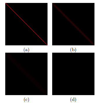
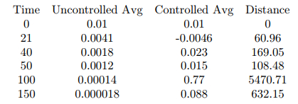
    In all the figures, red represents positive values and blue represents negative values. The uncontrolled simulation at 4 different timesteps: (a) 0, (b) 5, (c) 20 and (d) 100. The average value at the four timesteps: (a) 0.010, (b) 0.0079, (c) 0.0041 and (d) 0.00014

    .

    The control changes the weight at which a cell's evolution is impacted by the cells in its neigborhood. Since it is a scalar control there are only two possible transition rules though additional controls can be added to offer more flexibility as well as the possibility to impact only a subset of the cells in the grid. Figure 4 provides an example of controlled evolution with $ u(t) = {0if 0t<20 , 0t<50 or >t100 1otherwise

    $ and the coefficients $ \beta_{00} = 0, \beta_{10} = -0.34, \beta_{-10} = -0.24, \beta_{01} = -1.24 $ and $ \beta_{0-1} = -0.24 $.

    Figure 4. 

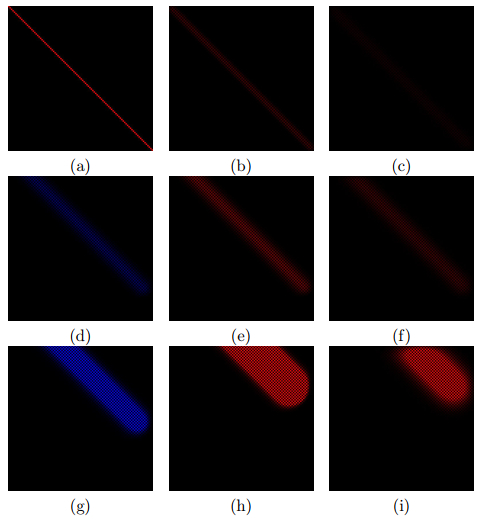
    The pictures show a controlled simulation at the following timesteps: (a) 0, (b) 5, (c) 20, (d) 39, (e) 40, (f) 50, (g) 75, (h) 100 and (i) 150. The control switches on at 20, off at 40, back on at 50 and finally off again at 100. Notice that while the control is off, the sign is constant and the magnitude diminishes at a slow exponential rate. When the control is on, the sign alternates with each timestep and the magnitude increases at a slow exponential rate

    .

    Section 4 provides additional examples with fire spreading and biological cell's growth.

    Definition 3.1. A cellular automaton is said to be controllable if for any initial $ s(0) = s_0 $ and final $ s(T) = s_T $ configurations, $ T<\infty $, there exists a control $ u $ such that $ s_T = Evol_T^{s_0, u} $.

    In the sequel we will therefore focus on situations where the control acts in specific ways. This is the case when for instance:

    ● the control can act only on a subset of the set of cells in the grid;

    ● the control is bounded;

    ● the value a control can take on one component of a state is constant over all cells in the grid;

    ● etc.

    For instance, the control can act on the grid as:

    $ Btut
    $
    (21)

    where $ B_t $ is an $ k\times l $ matrix and $ u_t $ is a $ l\times 1 $ vector. The matrix $ B_t $ indicates how the control is acting on the $ k $ components of the state of cell $ c $ ($ B_t\equiv 0 $ means that no control is applied to $ c $ at time $ t $) and $ u_t $ takes its value in the control domain (determined by the application) which is a subset of $ \mathbb R ^l $.

    Figure 5. 

    The average is negative for the odd numbered timesteps for which the control is active. For reference, the distance from the controlled simulation at timestep 150 to a grid of zeros is 632.06

    .

    To find a general framework to study the controllability problem, we will express our cellular automaton as a discrete control system. We introduce a configuration vector $ q $ that represents the value of each component of the state of a cell for all cells in the square lattice $ G $. Since the state of a cell has $ k $ components and we assume the grid is $ m\times m $, our state vector $ q $ belongs to a subset $ ( \mathbb R ^m\times \mathbb R ^m)^k $ which is determined by the state constraints. We introduce $ n = m^2k $ the dimension of vector $ q $. The global dynamics can then be written as:

    $ qt+1=F(qt,ut).
    $
    (22)

    Assume first that the control is fixed to 0 ($ u\equiv 0 $), the evolution of the system is governed by the uncontrolled transition function (13). Our system can be written as a linear discrete-time system:

    $ qt+1=Atqt+Btut,q0=initialconfiguration.
    $
    (23)

    where $ A_t $ is a $ n\times n $ matrix, $ B_t $ is a $ n\times l $ matrix and $ l $ the dimension of the control (typically a multiple of $ k $ as in section 4.1). The $ A $ matrix is typically a sparse matrix since the non zero elements occur only through the notion of neighbors, and in most problems the rules of the uncontrolled transition function do not depend on time, which makes $ A $ constant. When both $ A $ and $ B $ are constants, the system is said to be time invariant. Clearly, we have the following result.

    Proposition 1. The solution to (23) is given by:

    $ qt=ϕ(t,0)q0+t1j=0ϕ(t,j+1)Bjuj
    $
    (24)

    where the state transition matrix $ \phi(t, j) $ is defined by

    $ ϕ(t,j)={Iift=jAt1At2Ajotherwise
    $
    (25)

    Time Invariant System In this case the solution is given by

    $ qt=Atq0+t1j=0Atj1Buj
    $
    (26)

    where $ A^i $ denotes the matrix $ A $ to the power $ i $. Assume that $ A $ is diagonalizable, which means that there is an invertible matrix $ P $ such that $ A = PDP^{-1} $ and $ D $ is diagonal. A necessary and sufficient condition is that $ A $ has $ n $ linearly independent eigenvectors which is true in particular if $ A $ is symmetric. The uncontrolled state trajectory, also refereed to as the natural response, is then given by:

    $ qt=Atq0=PDtP1q0=nl=1βlλtlvl
    $
    (27)

    where $ \lambda_l $ are the eigenvalues of $ A $ associated to the eigenvectors $ v_l $ and the coefficient vector $ \beta = (\beta_1, \cdots, \beta_{n})^t $ is given by the initial condition $ q_0 $ when solving $ \beta = P^{-1}q_0 $, $ P = (v_1, \cdots, v_{n})^t $.

    We have well-known results about controllability for discrete linear systems, they translate to CA as follows.

    Proposition 2. A cellular automaton is controllable if and only if

    $ rank[An1B,An2B,,B]=n
    $
    (28)

    where $ A $ describes the uncontrolled transition function and $ B $ the action of the control. If $ A $ is diagonalizable, $ A = PDP^{-1} $, then the condition becomes $ {\rm rank}[D^{n-1}\tilde B, D^{n-2}\tilde B, \cdots, \tilde B] = n $ where $ \tilde B = P^{-1}B $.

    Example 4. We continue here example 3. In this case, we have that the state of our discrete linear system is given by:

    $ q=(s(c11),,s(c1m),s(c21),,s(c2m),,s(cm1),,s(cmm))
    $
    (29)

    and $ q_{t+1}(c_{ii}) = F(q_t(N_V^1(c_{ii}))) $ where $ F $ is deduced from (19). The matrix $ A $ corresponding to the natural response is given by:

    $ A = \left[ A1D20000D3A1D20000D3A1D20000D20000D3A1D20000D3A1
    \right] $

    where $ A_1 $ is an $ m\times m $ tri-diagonal matrix, and $ D_2, D_3 $ are $ m\times m $ diagonal matrices given by:

    $ A1=(abcabcbca),
    $
    (30)
    $ D2=(dd),D3=(ee)
    $
    (31)

    where to simplify the notations we introduced $ a = \alpha_{0, 0}, b = \alpha_{1, 0}, c = \alpha_{-1, 0}, d = \alpha_{0, 1}, e = \alpha_{0, -1} $. $ A $ is given by a band matrix and the evolution function $ Evol_T^{s_0} $ of this uncontrolled system is determined by the eigenvalues of the matrix $ A $. Table 1 contains the eigenvalues when assuming $ m = 5 $. It can be clearly seen by taking the limit of $ e $ and $ d $ when they tend to zero that the 25 eigenvalues collapse to the five eigenvalues of the first column when $ e = d = 0 $. Notice that depending on the sign of the coefficients $ a, b, c, d, e $ the eigenvalues might be complex.

    Table 1. 

    Eigenvalues corresponding to Example 4 and $ m = 5 $

    .
    $ a $ $ a\pm \sqrt{ed} $ $ a\pm \sqrt{3ed} $
    $ a+\sqrt{bc} $ $ a + \sqrt{bc+de\pm 2\sqrt{bcde}} $ $ a + \sqrt{bc+3de\pm2\sqrt{3bcde}} $
    $ a-\sqrt{bc} $ $ a - \sqrt{bc+de\pm 2\sqrt{bcde}} $ $ a - \sqrt{bc+3de\pm 2\sqrt{3bcde}} $
    $ a+\sqrt{3bc} $ $ a+\sqrt{3bc+3de\pm 6\sqrt{bcde}} $ $ a+\sqrt{3bc+3de+2\sqrt{3bcde}} $
    $ a-\sqrt{3bc} $ $ a-\sqrt{3bc+3de\pm 6\sqrt{bcde}} $ $ a-\sqrt{3bc+3de+2\sqrt{3bcde}} $

     | Show Table
    DownLoad: CSV

    We define the origin of a CA has the configuration with zeroes in all grid elements, and we have the following proposition.

    Proposition 3. The origin of the CA is asymptotically stable for the uncontrolled system if and only if $ |\lambda_i|<1 $ for all $ i = 1, \cdots, n $ where $ \lambda_i $ are the eigenvalues of $ A $. It is unstable if there exists an eigenvalue $ |\lambda_i|>1 $.

    Proof. This is a direct consequence from the fact that if the largest eigenvalue of a linear discrete control system is strictly less than 1, then the origin is asymptotically stable [3].

    In particular for our example with $ m = 5 $ assume that the coefficients of the transition function are all positive, and such that $ a+\sqrt{3bc+3de+ 6\sqrt{bcde}}<1 $, then the origin is asymptotically stable. In other words, the CA converges toward the equilibrium solution corresponding to a zero state value in each grid element. If $ a = 0.4, b = 0.2, c = 0.1, e = d = 0.1 $, then $ \max_{i} |\lambda_i| = 0.8537<1 $ and the origin is asymptotically stable. Assume the initial configuration is such that every grid element has state 10. After 30 time steps every state for our CA is less than $ 0.1 $ and after 90 time steps it is less than $ 10^{-6} $. Choosing the parameters as $ a = 0.4, b = 0.2, c = 0.4, e = d = 0.2 $ we have that the largest eigenvalue is $ 1.23 $ and therefore strictly greater than 1. The origin is then unstable. It can be seen through simulations, indeed if we choose the same initial configuration as before (state value of 10 in each grid element) after 20 iteration all states are greater than 150, they are all increasing rapidly.

    The following proposition highlights a surprising result stating that under some conditions a time invariant linear CA is controllable by controlling a single grid element only.

    Proposition 4. Assume $ e = d $ and all eigenvalues of $ A $ being distinct. We also assume that $ P^{-1} $ has at least a column with non zero values. Then, the CA is controllable with a scalar control on only one of the cell's grid.

    Proof. Since $ e = d $, $ A $ is diagonalizable and we assume $ \lambda_i\neq \lambda_j $ for $ i\neq j $ where $ \lambda_i $ are the eigenvalues. The rank condition $ {\rm rank}[D^{n-1}\tilde B, D^{n-2}\tilde B, \cdots, \tilde B] = n $ is equivalent to the Vandermonde matrix $ V = \left (1λ1λn111λ2λn121λnλn1n

    \right ), $ being invertible. Since det$ V = \Pi_{1\leq i<j\leq n}(\lambda_j-\lambda_i) $ it is non zero and controllability is guaranteed for any $ n\times 1 $ vector $ \tilde B $ with nonzero components. By construction $ \tilde B = P^{-1}B $ where $ P $ is the matrix of eigenvectors. If $ P^{-1} $ has a column non zero values, let us say column $ r $, then we simply set the $ r $-component of B to 1 and $ \tilde B $ satisfies the requirement.

    The CA model presented here is a generalization of typical cellular automaton applied to fire spreading where each cell is in only one of the following state: not flammable; the fuel cell unburned; burning cell; burned cell), and the rules are based on the neighborhood (Moore or Von Neumann) states and probabilities. Wind or external events can be incorporated in the transition rules through the use of control functions. In our model a cell can be in more than one stage with a fraction of it that can be burning and the rest of the cell already burned, moreover the external parameters can be controlled and their impact understood.

    The state of a cell $ c $ is given by four values: $ s_0(c) $ is the not flammable part of the cell, $ s_1(c) $ represents the fraction of the cell that is not touched by the fire (not burning nor burned), $ s_2(c) $ is the fraction of the cell that is burning and $ s_3(c) $ the fraction that is burned. Clearly we have that $ \sum_{i = 0}^3 s_i(c) = 1 $ since it represents 100% of the cell, $ s_i(c)\geq 0 $ for all $ i $ and the not flammable part of the cell is constant throughout the evolution of the fire unless there is an external action. Therefore, we have $ S\subseteq [0, 1]^4 $.

    The transition function is defined as follows:

    $ s0,t+1(c)=                         s0,t(c)
    $
    (32)
    $ s1,t+1(c)=              s1,t(c)[α1s2,t(c)+α2cN1V(c),ccs2,t(c)]s1,t(c)
    $
    (33)
    $ s2,t+1(c)=   s2,t(c)+(α1s1,t(c)α3)s2,t(c)+α2s1,t(c)cN1V(c),ccs2,t(c)
    $
    (34)
    $ s3,t+1(c)=                           s3,t(c)+α3s2,t(c)
    $
    (35)

    where $ \alpha_1 s_{1, t}(c)s_{2, t}(c) $ represents the fraction of untouched cell that starts burning due to existing fire in the central cell, $ \alpha_2 \sum\limits_{c'\in N_V^1(c), c'\neq c} s_{2, t}(c')s_{1, t}(c) $ is the fraction of untouched cell that starts burning due to fire in neighbouring cells and $ \alpha_3 s_{2, t}(c) $ depicts the quantify of burning land that is now completely burned. By definition the state constraint $ \sum_{i = 1}^4 s_i(c) = 1 $ is always satisfied (provided it is satisfied by the initial conditions) and the state's components are positive provided that $ 1\geq \alpha_1+\alpha_2 $ and $ 1\geq\alpha_3 $. It is a discrete model with linear and quadratic terms.

    The uncontrolled fire spreading CA can be written as a discrete control system as follows:

    $ qt+1=Aqt+QtHqt
    $
    (36)

    where the second terms represents the quadratic part of the transition rules, see equations (33-35). The matrix $ A $ is a block diagonal matrix:

    $ A=(A1000A1000000A1),A1=(10000100001α3000α31)
    $
    (37)

    which is invertible with determinant $ (1-\alpha_3)^{m^2} $ and $ A^{-1} $ is block diagonal with $ A_1^{-1} = \frac{1}{1-\alpha_3}\left (1α300001α300001000α31α3

    \right ) $. For the quadratic part, $ Q^t = (Q_1^t, \cdots, Q_{4m^2}^t) $ is a $ 4m^2\times (4m^2)^2 $ with all the elements of the square matrices $ Q_i^t $, $ i = 1, \cdots, n $ being equal to zero except the $ i -th $ line, which equals $ q^t $ and $ H = (H_1, \cdots, H_{4m^2}) $ is a $ (4m^2)^2\times 4m^2 $ matrix with each $ H_i $ constant with mostly zeroes but some $ \alpha_1 $ and $ \alpha_2 $ based on the transition rules.

    Remark 1. In our model, we consider $ N_V^1 $ but generalizations are easy, for instance to the Moore neighborhood. Indeed, we could simply add a term in (33) (and then substract it in 35) of the form $ \alpha_M \sum\limits_{c''\in N_M^1(c)\backslash N_V^1(c)} s_{1, t}(c') $ with $ \alpha_4<\alpha_2 $ to reflect that cells on fire that are in diagonal of the central one will have less impact for the central cell to get on fire than the adjacent ones. We also would need to adjust the condition on the coefficients to be $ 1\geq \alpha_1+\alpha_2+\alpha_4 $.

    Below we provide some simulations for our CA of fire spreading. Using the red-green-blue (RGB) color model, we represent the amount of burning material with the red component, the amount of flammable unburnt material with the green component and the amount of burnt material with the blue component. Thus, the amount of inflammable material can be inferred from the luminosity of the color.

    First, we compare the two different basic neighborhoods – the Von Neumann neighborhood and the Moore neighborhood. In Figure 6, we present two simulations, both of which start with a single location that is partially burning. As the two simulations progress, the different shapes that result from the two different neighborhoods become clear. It should be noted that the Moore neighborhood progresses much faster due to having more neighbors. Thus, the neighbor contribution is much greater. At timestep 50, the distance (as defined above) between the states of the two simulations is 6346.67. The timestep of the Moore neighborhood simulation that is closest to timestep 50 of the Von Neumann simulation is timestep 29 with a distance of 352.89.

    Figure 6. 

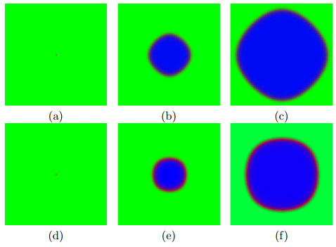
    Top row using the Von Neumann neighborhood. Timesteps: (a) 1, (b) 50 and (c) 100. Bottom row using the Moore neighborhood. Timesteps: (a) 1, (b) 25 and (c) 50. Note that the Moore neighborhood promotes much faster evolution. For both $ \alpha_1 = 0.1 $, $ \alpha_2 = 0.2 $ and $ \alpha_3 = 0.3 $

    .

    Next, we compare different values of the $ \alpha_i $'s and the effect it has on the rate of spreading as well as the width of the burning band (see Figure 7). For all the remaining fire simulations, we use the Von Neumann neighborhood. These two simulations rapidly diverge. By timestep 10 the distance between them is 147.54, by timestep 50 the distance is 4853.13 and by timestep 100 the distance is 15504.70.

    Figure 7. 

    Top row: $ \alpha_1 = 0.05 $, $ \alpha_2 = 0.1 $ and $ \alpha_3 = 0.15 $. Bottom row: $ \alpha_1 = 0.15 $, $ \alpha_2 = 0.3 $ and $ \alpha_3 = 0.05 $. For both, the three times steps are 1, 50 and 100

    .

    For this example the control can be viewed as as an external input in the form of any treatment applied directly to burning fuel (wetting, smothering, or chemically quenching the fire) or by physically separating the burning from not burned fuel (done by fire engines, fire personnel and aircraft applying water or fire retardant directly to the burning fuel). It can also correspond to creating control lines: boundaries that contain no combustible material or by using fire retardants, fire-fighting foams, and superabsorbent polymer gels. These can clearly act on either of our three component of the state (independently or at the same time). The conditions for controllability are more complex than in the linear case, but since the matrix $ H $ is sparse the problem is easier. It will be studied in forthcoming work.

    Assume we have the capability to build a barricade which for us translates into act on the fraction of the fuel cell unburned and turn it into a not flammable component. This means that we need to introduce a control that will grow $ s_{0, t}(c) $ by the amount $ s_{1, t}(c) $ and put the latter one to zero (for simplicity we do not consider the case when only a fraction of the fuel cell unburned is turned into not flammable since it is a straightforward extension but makes the equations unnecessarily more complicated). This means that for the cells that can be affected by a barricade, the controlled transfer function is now:

    $ s0,t+1(c)=               s0,t(c)+u0,t(c)s1,t(c)
    $
    (38)
    $ s1,t+1(c)=     [s1,t(c)f10(s1,t(c),s2,t(c),s2,t(c))](1u0,t(c))
    $
    (39)
    $ s2,t+1(c)=   (1α3)s2,t(c)+f10(s1,t(c),s2,t(c),s2,t(c))(1u0,t(c))
    $
    (40)
    $ s3,t+1(c)=             s3,t(c)+α3s2,t(c)
    $
    (41)

    where $ f_0^1 $ is given by (33-35), $ c'\in N_V^1(c), c'\neq c $, and $ u_{0, t}(c)\in \{0, 1\} $. If $ u_{0, t}(c) = 0 $ it corresponds to the natural evolution, however when $ u_{0, t}(c) $ is turned to 1 no more fire can take place in cell $ c $ which corresponds to the barricade being constructed.

    We will consider two examples involving barricades. Computationally, a barricade is simply a region in which combustible material, burning material and burnt material are all zero. The first example, shown in Figure 8, we consider a fixed obstacle and we can see how the spreading fire has to divert around the obstacle. This increases the amount of time it takes to reach locations on the far side of the obstacles, but does not seem to have significant long-term impacts on the shape of the fire. Second, we consider the siutation where an obstacle (or sequence of obstacles) is introduced as the fire progresses. Notice that in Figure 9 a small region of fire appears to materialize on the far side of the barricade. This is due to the fact that, although it is not visible, by timestep 20, the fire has already reached beyond the barricade. After a short period of time, that small amount of fire has grown to a visible level. Creating barricades as the simulation progresses is one of the two types of control we consider.

    Figure 8. 

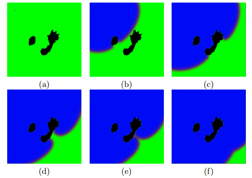
    Timesteps: (a) 1, (b) 125, (c) 175, (d) 200, (e) 210 and (f) 250. The fire is diverted by the obstacles

    .
    Figure 9. 

    Timesteps: (a) 1, (b) 20, (c) 30, (d) 38, (e) 45 and (f) 100. The fire is diverted by the obstacles

    .

    Let us assume now that we can put the fire down in a region (which is equivalent to a subset of the cell in the grid), this means that no new fire will take place in such cell at that moment and the fire will go extinct. However, it does not convert the "fuel" fraction of the cells into not flammable. The control would then be introduced as follow:

    $ s0,t+1(c)=                     s0,t(c)
    $
    (42)
    $ s1,t+1(c)=     s1,t(c)f10(s1,t(c),s2,t(c),s2,t(c))(1u2,t(c))
    $
    (43)
    $ s2,t+1(c)=  [(1α3)s2,t(c)+f10(s1,t(c),s2,t(c),s2,t(c))](1u2,t(c))
    $
    (44)
    $ s3,t+1(c)=         s3,t(c)+(α3(1u2,t(c))+u2,t(c))s2,t(c)
    $
    (45)

    where $ u_{2, t}(c)\in \{0, 1\} $ controls fire extinction.

    We illustrate this second form of control with a simulation starting from the same initial conditions. In Figure 10, we extinguish the fire in a small region at timestep 20. Notice that this has more significant long-term consequences on the shape of the spreading fire than obstacles. Also, notice the darker region which remains after the fire has passed. This artifact results from extinguishing an active fire, therefore reducing the total amount of material in the region.

    Figure 10. 

    Timesteps: (a) 1, (b) 20, (c) 25, (d) 35, (e) 50 and (f) 100. The fire is diverted by the obstacles

    .

    In our model, the topographical organization of fractone expression reflects the shaping of the mass of cells. We hypothetize that the fractones guide the shape of multicellular organisms, therefore the cellular automaton must capture the interplay between the different types of cells and the fractones playing the role of chemical effector for the molecular mechanisms that control stem-cell fate. The CA in [2] was designed as two automata co-evolving in parallel and feeding each other with information to adjust the corresponding transition functions. One automaton, the diffusion automaton, was accounting for the evolution of the growth factors, and the second automaton, the mitosis automaton, was designed with a transition function depicting rules for cells division. In this paper, as a first step to develop control strategies to grow specific forms we neglect the growth factors and their diffusion process. Indeed, it was shown in [2] that the growth factor diffusion mainly controls the time scale of cell growth and that the fractones are dominant in determining shape. The main difficulty is to combine a fixed duration and a dynamic spatial location of the fractones during that duration that will bring an initial mass of cell to a desired one. The fact that the evolution has to occur over a prescribed time frame is key in morphogenesis.

    We introduce the state of a grid cell as a single value between 0 and 1. If $ 0 \leq s(c)<1 $ it is considered that no biological cell is present in the corresponding unit $ c $ of the grid, and $ s(c) = 1 $ means the existence of a biological cell. Intuitively, when $ s(c)\in (0, 1) $ the state expresses the probability that a biological cell will be present in the next time step. The transition rule for the uncontrolled process is for $ c\in G $:

    $ st+1(c)=max{1,st(c)+ciN(c)αt(c,ci)st(ci)}
    $
    (46)

    where $ \alpha_t(c, c_i) $ is some constant depending on the organism under consideration. It captures the "natural" growth of a cellular mass without the action of fractones. Here the coefficients depend on time, indeed once there is a biological cell, i.e. $ s_t(c) = 1 $ the state of the cell does not evolve, unless there is an external event, which is expressed by $ \alpha_t(c, c_i) = 0 $ for all $ c_i\in N(c) $ in that case. Note that contrary to the other example and the fire application, we have for this example a state constraint by imposing $ s_{t+1}(c)\leq 1 $.

    The neighborhood can be chosen in various ways depending again on the organism under study and the stage of the cellular mass under consideration (adult or embryo). In Figure 11, we illustrate a simple example of cell growth, starting from one cell and using the standard Von Neumann neighborhood. We contrast this with Figure 14 in which we use a non-standard neighborhood to acheive markedly different results. Although we do not illustrate this here, we also admit the possibility that the choice of neighborhood may vary with time or even be used as a control mechanism.

    Figure 11. 

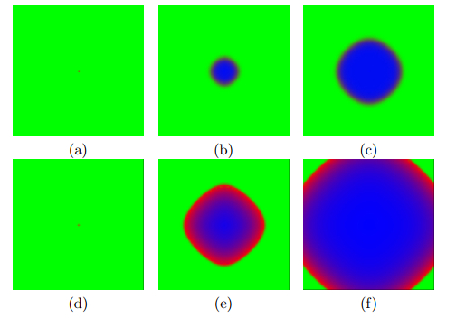
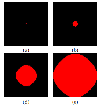
    Timesteps: (a) 1, (b) 15, (c) 50 and (d) 100. A simple, uncontrolled cell growth using the Von Neumann neighborhood

    .
    Figure 12. 

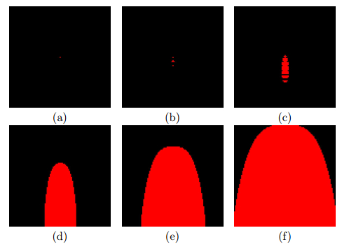
    Timesteps: (a) 1, (b) 5, (c) 10, (d) 30, (e) 60 and (f) 100. An uncontrolled cell growth using a neighborhood consisting of the three grid units directly above the central unit and the three side-by-side units in the row three rows below the central unit

    .
    Figure 14. 

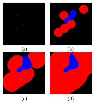
    Timesteps: (a) 0, (b) 30, (c) 60 and (d) 100. The interaction between growth of normal cells and tumor cells. The competition between the cell masses plays out at the boundary between the cell masses. The normal cells are in red, the probability of a tumor cell developing is in blue

    .

    The natural growth without the introduction of fractones will provide a growth directed by the constants $ \alpha_t(c, c_i) $, in particular if we start with one cell and we assume the coefficients $ \alpha_t(c, c_i) $ do not depend on $ c_i $ but are all the same for every cell in the neighborhood we will grow a isotropic mass (see Figure 11).

    To break the symmetry and create more sophisticated masses of cells we must activate the controls (playing solely with the notion of neighborhood is not fine enough and does not reflect our biological hypothesis). The controls are: the fractones that can accelerate or decelerate growth; and spontaneous death for the cells.

    Definition 4.1. If a fractone is associated to a cell, then its corresponding coefficient in the transition function is altered either by an increasing factor if the fractone is inducing accelerated growth, in which case we call it a positive fractone, or by a decreasing factor if the fractone is decelerating growth which is then called a negative fractone.

    More precisely, we have the following. Assume $ c_j $ such that $ s_t(c_j) = 1 $, i.e. there is a biological cell in that grid unit, and that we have a positive fractone associated to this biological cell. We introduce $ u^+_t(c_j) $ a positive real number and the coefficients $ \alpha_t(c, c_j) $ are replaced by $ \alpha_t(c, c_j)+u^+_t(c_j) $ in all transition rules that involve $ c_j $. In particular, if $ c_j $ is in the neighborhood of $ c $, we have:

    $ st+1(c)=max{1,st(c)+cicjN(c)αt(c,ci)st(ci)+(αt(c,cj)+u+t(cj))st(cj)}
    $
    (47)

    The value $ u^+_t(c_i) $ depends on the chemical composition of that specific fractone. The transition rule is modified the same way for negative fractones with the constraint that $ \alpha_t(c, c_j)-u^-_t(c_j)\geq 0 $, $ u^-_t(c_j) $ is a positive real number.

    The present model can be described in terms of a discrete control system as follows. Assume the possible chemical composition of positive fractones is captured by $ l $ positive real numbers (i.e. there is a finite number of speed at which fractones can accelerate growth), and similarly for negative fractones we assume their possible chemical composition is given by a finite vector of length $ s $: $ \beta^+\in \mathbb R ^l, \beta^-\in \mathbb R ^s $. Assume the dimension of the state vector $ q $ to be $ n $, we then have:

    $ qt+1=Atqt+U+tβ++Utβ,0qt+11
    $
    (48)

    where $ A_t $ is an $ n\times n $ matrix that represents the natural growth, and $ U^+ $ (resp. $ U^- $) is a $ n\times l $ (resp. $ n\times s $) control matrix whose entries are binary, 0 or 1, with 1 representing the existence of a positive (resp. negative) fractone. Notice that the control part does not include the state since fractones are associated to existing cells and therefore only to $ c_j $ such that $ s_t(c_j) = 1 $. The value of $ u^+_t(c_j)) $ ($ u^-_t(c_j) $) is deduced from $ U^+_t\beta^+ $ ($ U^-_t \beta^- $).

    In Figure 13, we illustrate the affect that the fractones can have on the shape of the results. One line of fractones increases the rate of growth and results in the oblong shape of the cell mass. Below that is a line of fractones that stop cell growth. Notice that these hardly have any impact on the shape, except that they stop cell growth at their locations. Above the first line is a row of blocks of fractones that stop cell growth. These have some impact on the shape of the cell mass simply because they act as an barricade, much like the barricades in the fire simulations.

    Figure 13. 

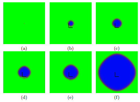
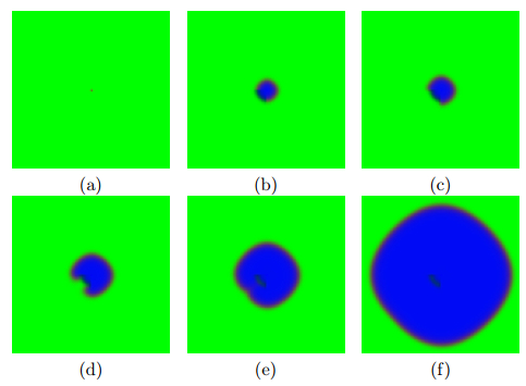
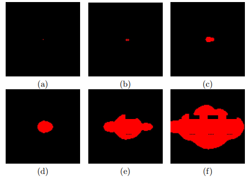
    Timesteps: (a) 1, (b) 5, (c) 15, (d) 30, (e) 60 and (f) 100. Fractones are placed along three horizontal lines. One is above the initial cell and consists of fractones that stop cell growth; they are arranged in blocks. One is in line with the initial cell (across the middle of the simulation) and greatly increases cell growth. The final line is below the intial cell and also stops cell growth. The placement of the fractones is clearly visible in (f)

    .

    Definition 4.2. Death of cell can occur in a spontaneous way. If a biological cell exists in grid unit $ c $, i.e. $ s_t(c) = 1 $, the death of this specific cell means that its state reset to the value zero: $ s_{t+1}(c) = 0 $.

    By definition the control corresponding to cell's death is a vector $ u^d_t\in \mathbb R ^n $ whose entries are zero for state components $ q_t^i $ that are not equal to 1 or correspond to an existing biological cell not dying, and are 1 for grid units with a biological cell undergoing spontaneous death. The system becomes:

    $ qt+1=Atqt+U+tβ++Utβ+udt,0qt+11.
    $
    (49)

    A single grid cell of our two dimensional lattices will be occupied by either an empty space, a cancer cell or a normal cell (not cancerous). The state for each grid cell is characterized by an ordered pair $ (s_1, s_2)\in [0, 1]^2 $ to mimic our model on cell's growth 4.2.1 where $ s_1 $ accounts for the probability to get a normal cell and $ s_2 $ for the probability to get a cancer cell. If $ s_{1, t} = 1 $ there is a biological cell in that grid unit and if $ s_{2, t} = 1 $ there is a tumor cell.

    The model is similar to that of cell growth, but a state is now a pair and the transition rules for the natural growth are as follows:

    $ s1,t+1(c)=max{1,s1,t(c)+ciN1(c)α1,t(c,ci)s1,t(ci)}
    $
    (50)
    $ s2,t+1(c)=max{1,s2,t(c)+ciN2(c)α2,t(c,ci)s2,t(ci)}
    $
    (51)

    with the additional state constraints:

    $ ifs1,t(c)=1,thens2,t(c)=0,
    $
    (52)
    $ ifs2,t(c)=1,thens1,t(c)=0.
    $
    (53)

    The coefficients $ \alpha $ are assumed such that $ \alpha_{2, t}(c, c_i)\geq \alpha_{1, t}(c, c_i) $ to express that a tumor cell will divide at a more rapid rate than normal cells. The constraints make explicit that if there is a normal biological cell in grid unit $ c $ then the cell cannot become a cancer cell and can only serve to influence its neighbours to become normal cells. Also, note that $ N_1 $ and $ N_2 $ might differ since the radius of influence of an aggressive tumor might be bigger than the one for healthy cells.

    The role of fractones in tumor growth is unclear at this stage, it would be however interesting to create a virtual lab to test different hypotheses with chemical composition and distribution of fractones related to the cancer cells.

    This paper is a first approach to apply discrete control theory to analyze the behavior of controlled cellular automata. The framework is designed to be flexible enough to allow for heterogeneity regarding the grid cell's states, indeed as it can be observed in the fire application for instance some areas might be set as completely inflammable while others are flammable or possibly at least partially. The heterogeneity distribution can also evolve with time, which is illustrated with the possibility to introduce obstacles throughout the evolution of the dynamical system under study. In the tumor growth application, different types of cells can be introduced to mimic organs various sensitivity to specific type of cancer.

    We presented how different control strategies affect the evolution of the system, and the next step will be to use more in depth results from discrete control systems to come-up with systematic ways to design control strategies to reach a final goal. It could be stabilize the size of the rumor for instance or determine the distribution of fractones to grow a specific form during fixed time period. In addition, in forthcoming work optimal control of discrete systems will be explorer to not only reach a prescribed goal but in the most efficient way given a cost. Based on this first approach, the authors are optimistic regarding the application of discrete control methods to this class of controlled cellular automata.


    [1] A cellular automaton model for tumour growth in inhomogeneous environment. Journal of Theoretical Biology (2003) 225: 257-274.
    [2]

    A. Beros, M. Chyba, A. Fronville and F. Mercier, A morphogenetic cellular automaton, in 2018 Annual American Control Conference (ACC), IEEE, 2018, 1987–1992.

    [3]

    A. B. Bishop, Introduction to Discrete Linear Controls: Theory and Application, Elsevier, 2014.

    [4] Cell-level finite element studies of viscous cells in planar aggregates. Journal of Biomechanical Engineering (2000) 122: 394-401.
    [5] Fractone-heparan sulphates mediate fgf-2 stimulation of cell proliferation in the adult subventricular zone. Cell Proliferation (2013) 46: 137-145.
    [6]

    S. El Yacoubi and P. Jacewicz, Cellular automata and controllability problem, in CD-Rom Proceeding of the 14th Int. Symp. on Mathematical Theory of Networks and Systems, june, 2000, 19–23.

    [7] Analyse et contrôle par automates cellulaires. Annals of the University of Craiova-Mathematics and Computer Science Series (2003) 30: 210-221.
    [8] Novel extracellular matrix structures in the neural stem cell niche capture the neurogenic factor fibroblast growth factor 2 from the extracellular milieu. Stem Cells (2007) 25: 2146-2157.
    [9] Emergence and control of macro-spatial structures in perturbed cellular automata, and implications for pervasive computing systems. IEEE Transactions on Systems, Man, and Cybernetics-Part A: Systems and Humans (2005) 35: 337-348.
    [10] Fractones: Extracellular matrix niche controlling stem cell fate and growth factor activity in the brain in health and disease. Cellular and Molecular Life Sciences (2016) 73: 4661-4674.
    [11] Bone morphogenetic protein-4 inhibits adult neurogenesis and is regulated by fractone-associated heparan sulfates in the subventricular zone. Journal of Chemical Neuroanatomy (2014) 57: 54-61.
    [12] Anatomy of the brain neurogenic zones revisited: Fractones and the fibroblast/macrophage network. Journal of Comparative Neurology (2002) 451: 170-188.
    [13] Adhesion between cells, diffusion of growth factors, and elasticity of the aer produce the paddle shape of the chick limb. Physica A: Statistical Mechanics and its Applications (2007) 373: 521-532.
    [14] An integrated agent-mathematical model of the effect of intercellular signalling via the epidermal growth factor receptor on cell proliferation. Journal of Theoretical Biology (2006) 242: 774-789.
  • Reader Comments
  • © 2019 the Author(s), licensee AIMS Press. This is an open access article distributed under the terms of the Creative Commons Attribution License (http://creativecommons.org/licenses/by/4.0)
通讯作者: 陈斌, bchen63@163.com
  • 1. 

    沈阳化工大学材料科学与工程学院 沈阳 110142

  1. 本站搜索
  2. 百度学术搜索
  3. 万方数据库搜索
  4. CNKI搜索

Metrics

Article views(6436) PDF downloads(472) Cited by(0)

Figures and Tables

Figures(14)  /  Tables(1)

/

DownLoad:  Full-Size Img  PowerPoint
Return
Return

Catalog