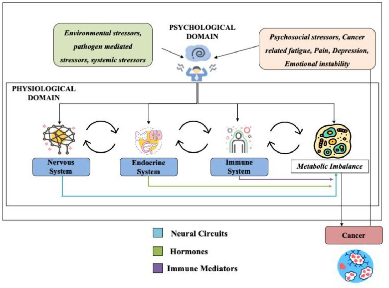
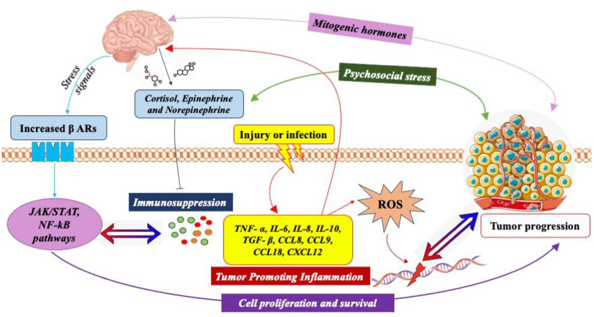
Neuroendocrine-immune homeostasis in health and disease is a tightly regulated bidirectional network that influences predisposition, onset and progression of age-associated disorders. The complexity of interactions among the nervous, endocrine and immune systems necessitates a complete review of all the likely mechanisms by which each individual system can alter neuroendocrine-immune homeostasis and influence the outcome in age and disease. Dysfunctions in this network with age or external/internal stimuli are implicated in the development of several disorders including autoimmunity and cancer. The existence of sympathetic noradrenergic innervations on lymphoid organs in synaptic association with immune cells that express receptors for endocrine mediators such as hormones, neural mediators such as neurotransmitters and immune effector molecules such as cytokines explains the complicated nature of the regulatory pathways that must always maintain homeostatic equilibrium within and among the nervous, endocrine and immune systems. The incidence, development and progression of cancer, affects each of the three systems by disrupting regulatory pathways and tipping the scales away from homeostasis to favour pathways that enable it to evade, override and thrive by using the network to its advantage. In this review, we have explained how the neuroendocrine-immune network is altered in female reproductive aging and cancer, and how these modulations contribute to incidence and progression of cancer and hence prove to be valuable targets from a therapeutic standpoint. Reproductive aging, stress-associated central pathways, sympathetic immunomodulation in the periphery, inflammatory and immunomodulatory changes in central, peripheral and tumor-microenvironment, and neuro-neoplastic associations are all likely candidates that influence the onset, incidence and progression of cancer.
Citation: Hannah P. Priyanka, Rahul S. Nair, Sanjana Kumaraguru, Kirtikesav Saravanaraj, Vasantharekha Ramasamy. Insights on neuroendocrine regulation of immune mediators in female reproductive aging and cancer[J]. AIMS Molecular Science, 2021, 8(2): 127-148. doi: 10.3934/molsci.2021010
Neuroendocrine-immune homeostasis in health and disease is a tightly regulated bidirectional network that influences predisposition, onset and progression of age-associated disorders. The complexity of interactions among the nervous, endocrine and immune systems necessitates a complete review of all the likely mechanisms by which each individual system can alter neuroendocrine-immune homeostasis and influence the outcome in age and disease. Dysfunctions in this network with age or external/internal stimuli are implicated in the development of several disorders including autoimmunity and cancer. The existence of sympathetic noradrenergic innervations on lymphoid organs in synaptic association with immune cells that express receptors for endocrine mediators such as hormones, neural mediators such as neurotransmitters and immune effector molecules such as cytokines explains the complicated nature of the regulatory pathways that must always maintain homeostatic equilibrium within and among the nervous, endocrine and immune systems. The incidence, development and progression of cancer, affects each of the three systems by disrupting regulatory pathways and tipping the scales away from homeostasis to favour pathways that enable it to evade, override and thrive by using the network to its advantage. In this review, we have explained how the neuroendocrine-immune network is altered in female reproductive aging and cancer, and how these modulations contribute to incidence and progression of cancer and hence prove to be valuable targets from a therapeutic standpoint. Reproductive aging, stress-associated central pathways, sympathetic immunomodulation in the periphery, inflammatory and immunomodulatory changes in central, peripheral and tumor-microenvironment, and neuro-neoplastic associations are all likely candidates that influence the onset, incidence and progression of cancer.

| [1] | Ader R, Felten DL, Cohen N (2001) Psychoneuroimmunology New York: Academic Press. |
| [2] |
Seifert P, Spitznas M (2001) Tumours may be innervated. Virchows Arch 438: 228-231. doi: 10.1007/s004280000306

|
| [3] |
Seifert P, Benedic M, Effert P (2002) Nerve fibers in tumors of the human urinary bladder. Virchows Arch 440: 291-297. doi: 10.1007/s004280100496
|
| [4] |
Lu SH, Zhou Y, Que HP, et al. (2003) Peptidergic innervation of human esophageal and cardiac carcinoma. World J Gastroenterol 9: 399-403. doi: 10.3748/wjg.v9.i3.399
|
| [5] | Liang YJ, Zhou P, Wongba W, et al. (2010) Pulmonary innervation, inflammation and carcinogenesis. Sheng Li Xue Bao 62: 191-195. |
| [6] |
Priyanka HP, ThyagaRajan S (2013) Selective modulation of lymphoproliferation and cytokine production via intracellular signaling targets by α1- and α2-adrenoceptors and estrogen in splenocytes. Int Immunopharmacol 17: 774-784. doi: 10.1016/j.intimp.2013.08.020
|
| [7] | Meites J, Quadri SK (1987) Neuroendocrine theories of aging. The Encyclopedia of Aging New York: Springer, 474-478. |
| [8] |
ThyagaRajan S, MohanKumar PS, Quadri SK (1995) Cyclic changes in the release of norepinephrine and dopamine in the medial basal hypothalamus: effects of aging. Brain Res 689: 122-128. doi: 10.1016/0006-8993(95)00551-Z
|
| [9] | ThyagaRajan S, Priyanka HP (2012) Bidirectional communication between the neuroendocrine system and the immune system: relevance to health and diseases. Ann Neurosci 19: 40-46. |
| [10] |
Mravec B, Gidron Y, Hulin I (2008) Neurobiology of cancer: interactions between nervous, endocrine and immune systems as a base for monitoring and modulating the tumorigenesis by the brain. Semin Cancer Biol 18: 150-163. doi: 10.1016/j.semcancer.2007.12.002
|
| [11] |
Mukhtar RA, Nseyo O, Campbell MJ, et al. (2011) Tumor-associated mac-rophages in breast cancer as potential biomarkers for new treatments and diagnostics. Expert Rev Mol Diagn 11: 91-100. doi: 10.1586/erm.10.97
|
| [12] |
Müller A, Homey B, Soto H, et al. (2001) Involvement of chemokine receptors in breast cancer metastasis. Nature 410: 50-56. doi: 10.1038/35065016
|
| [13] |
Hanahan D, Coussens LM (2012) Accessories to the crime: functions of cells recruited to the tumor microenvironment. Cancer Cell 21: 309-322. doi: 10.1016/j.ccr.2012.02.022
|
| [14] |
Hanahan D, Weinberg RA (2011) Hallmarks of cancer: the next generation. Cell 144: 646-674. doi: 10.1016/j.cell.2011.02.013
|
| [15] |
Cole SW, Nagaraja AS, Lutgendorf SK, et al. (2015) Sympathetic nervous system regulation of the tumour microenvironment. Nat Rev Cancer 15: 563-572. doi: 10.1038/nrc3978
|
| [16] |
Segerstrom SC, Miller GE (2004) Psychological stress and the human immune system: a meta-analytic study of 30 years of inquiry. Psychol Bull 130: 601-630. doi: 10.1037/0033-2909.130.4.601
|
| [17] |
Greten FR, Grivennikov SI (2019) Inflammation and cancer: triggers, mechanisms, and consequences. Immunity 51: 27-41. doi: 10.1016/j.immuni.2019.06.025
|
| [18] |
Yang H, Xia L, Chen J, et al. (2019) Stress-glucocorticoid-TSC22D3 axis compromises therapy-induced antitumor immunity. Nat Med 25: 1428-1441. doi: 10.1038/s41591-019-0566-4
|
| [19] |
Curtin NM, Boyle NT, Mills KH, et al. (2009) Psychological stress suppresses innate IFN-gamma production via glucocorticoid receptor activation: reversal by the anxiolytic chlordiazepoxide. Brain Behav Immun 23: 535-547. doi: 10.1016/j.bbi.2009.02.003
|
| [20] |
Key TJ (1995) Hormones and cancer in humans. Mutat Res 333: 59-67. doi: 10.1016/0027-5107(95)00132-8
|
| [21] |
Mravec B, Tibensky M, Horvathova L (2020) Stress and cancer. Part I: Mechanisms mediating the effect of stressors on cancer. J Neuroimmunol 346: 577311. doi: 10.1016/j.jneuroim.2020.577311
|
| [22] |
Yin W, Gore AC (2006) Neuroendocrine control of reproductive aging: roles of GnRH neurons. Reproduction 131: 403-414. doi: 10.1530/rep.1.00617
|
| [23] | Reed BG, Carr BR (2000) The Normal Menstrual Cycle and the Control of Ovulation. Endotext South Dartmouth (MA): MDText.com, Inc. |
| [24] |
Del Río JP, Alliende MI, Molina N, et al. (2018) Steroid Hormones and Their Action in Women's Brains: The Importance of Hormonal Balance. Front Public Health 6: 141. doi: 10.3389/fpubh.2018.00141
|
| [25] |
Djahanbakhch O, Ezzati M, Zosmer A (2007) Reproductive ageing in women. J Pathol 211: 219-231. doi: 10.1002/path.2108
|
| [26] | Braunwald E, Isselbacher KJ, Petersdorf RG, et al. (1987) Harrison's Principles of Internal Medicine New York: McGraw-Hill, 1818-1837. |
| [27] |
Priyanka HP, Nair RS (2020) Neuroimmunomodulation by estrogen in health and disease. AIMS Neurosci 7: 401-417. doi: 10.3934/Neuroscience.2020025
|
| [28] |
Sherman BM, West JH, Korenman SG (1976) The menopausal transition: analysis of LH, FSH, estradiol, and progesterone concentrations during menstrual cycles of older women. J Clin Endocrinol Metab 42: 629-636. doi: 10.1210/jcem-42-4-629
|
| [29] |
Hall JE, Gill S (2001) Neuroendocrine aspects of aging of aging in women. Endocrinol Metab Clin North Am 30: 631-646. doi: 10.1016/S0889-8529(05)70205-X
|
| [30] |
Lang TJ (2004) Estrogen as an immunomodulator. Clin Immunol 113: 224-230. doi: 10.1016/j.clim.2004.05.011
|
| [31] |
Salem ML (2004) Estrogen, a double-edged sword: modulation of TH1- and TH2-mediated inflammations by differential regulation of TH1/TH2 cytokine production. Curr Drug Targets Inflamm Allergy 3: 97-104. doi: 10.2174/1568010043483944
|
| [32] |
Wise PM, Scarbrough K, Lloyd J, et al. (1994) Neuroendocrine concomitants of reproductive aging. Exp Gerontol 29: 275-283. doi: 10.1016/0531-5565(94)90007-8
|
| [33] |
Chakrabarti M, Haque A, Banik NL, et al. (2014) Estrogen receptor agonists for attenuation of neuroinflammation and neurodegeneration. Brain Res Bull 109: 22. doi: 10.1016/j.brainresbull.2014.09.004
|
| [34] |
ThyagaRajan S, Madden KS, Teruya B, et al. (2011) Age-associated alterations in sympathetic noradrenergic innervation of primary and secondary lymphoid organs in female Fischer 344 rats. J Neuroimmunol 233: 54-64. doi: 10.1016/j.jneuroim.2010.11.012
|
| [35] |
Teilmann SC, Clement CA, Thorup J, et al. (2006) Expression and localization of the progesterone receptor in mouse and human reproductive organs. J Endocrinol 191: 525-535. doi: 10.1677/joe.1.06565
|
| [36] |
Butts CL, Shukair SA, Duncan KM, et al. (2007) Progesterone inhibits mature rat dendritic cells in a receptor-mediated fashion. Int Immunol 19: 287-296. doi: 10.1093/intimm/dxl145
|
| [37] |
Jones LA, Kreem S, Shweash M, et al. (2010) Differential modulation of TLR3- and TLR4-mediated dendritic cell maturation and function by progesterone. J Immunol 185: 4525-4534. doi: 10.4049/jimmunol.0901155
|
| [38] |
Menzies FM, Henriquez FL, Alexander J, et al. (2011) Selective inhibition and augmentation of alternative macrophage activation by progesterone. Immunology 134: 281-291. doi: 10.1111/j.1365-2567.2011.03488.x
|
| [39] |
Hardy DB, Janowski BA, Corey DR, et al. (2006) Progesterone receptor plays a major antiinflammatory role in human myometrial cells by antagonism of nuclear factor-κB activation of cyclooxygenase 2 expression. Mol Endocrinol 20: 2724-2733. doi: 10.1210/me.2006-0112
|
| [40] |
Arruvito L, Giulianelli S, Flores AC, et al. (2008) NK cells expressing a progesterone receptor are susceptible to progesterone-induced apoptosis. J Immunol 180: 5746-5753. doi: 10.4049/jimmunol.180.8.5746
|
| [41] | Piccinni MP, Giudizi MG, Biagiotti R, et al. (1995) Progesterone favors the development of human T helper cells producing TH2-type cytokines and promotes both IL-4 production and membrane CD30 expression in established TH1 cell clones. J Immunol 155: 128-133. |
| [42] |
Özdemir BC, Dotto GP (2019) Sex hormones an anticancer immunity. Clin Cancer Res 25: 4603-4610. doi: 10.1158/1078-0432.CCR-19-0137
|
| [43] |
Beral V (2003) Breast cancer and hormone-replacement therapy in the Million Women Study. Lancet 362: 419-427. doi: 10.1016/S0140-6736(03)14596-5
|
| [44] |
Grady D, Gebretsadik T, Kerlikowske K, et al. (1995) Hormone replacement therapy and endometrial cancer risk: a meta-analysis. Obstet Gynecol 85: 304-313. doi: 10.1016/0029-7844(94)00383-O
|
| [45] |
Lacey JV, Mink PJ, Lubin JH, et al. (2002) Menopausal hormone replacement therapy and risk of ovarian cancer. JAMA 288: 334-341. doi: 10.1001/jama.288.3.334
|
| [46] |
Fournier A, Berrino F, Clavel-Chapelon F (2008) Unequal risks for breast cancer associated with different hormone replacement therapies results from the E3N cohort study. Breast Cancer Res Treat 107: 103-111. doi: 10.1007/s10549-007-9523-x
|
| [47] |
Anderson GL, Limacher M, Assaf AR, et al. (2004) Effects of conjugated equine estrogen in postmenopausal women with hysterectomy: the Women's Health Initiative randomized controlled trial. JAMA 291: 1701-1712. doi: 10.1001/jama.291.14.1701
|
| [48] |
Key TJ, Pike MC (1988) The dose-effect relationship between ‘unopposed’ oestrogens and endometrial mitotic rate: its central role in explaining and predicting endometrial cancer risk. Br J Cancer 57: 205-212. doi: 10.1038/bjc.1988.44
|
| [49] |
Cook MB, Dawsey SM, Freedman ND, et al. (2009) Sex disparities in cancer incidence by period and age. Cancer Epidemiol Biomarkers Prev 18: 1174-1182. doi: 10.1158/1055-9965.EPI-08-1118
|
| [50] |
Cook MB, McGlynn KA, Devesa SS, et al. (2011) Sex disparities in cancer mortality and survival. Cancer Epidemiol. Biomarkers Prev 20: 1629-1637. doi: 10.1158/1055-9965.EPI-11-0246
|
| [51] |
Lista P, Straface E, Brunelleschi S, et al. (2011) On the role of autophagy in human diseases: a gender perspective. J Cell Mol Med 15: 1443-1457. doi: 10.1111/j.1582-4934.2011.01293.x
|
| [52] |
Lin PY, Sun L, Thibodeaux SR, et al. (2010) B7-H1-dependent sex-related differences in tumor immunity and immunotherapy responses. J Immunol 185: 2747-2753. doi: 10.4049/jimmunol.1000496
|
| [53] |
Polanczyk MJ, Hopke C, Vandenbark AA, et al. (2006) Estrogen-mediated immunomodulation involves reduced activation of effector T cells, potentiation of Treg cells, and enhanced expression of the PD-1 costimulatory pathway. J Neurosci Res 84: 370-378. doi: 10.1002/jnr.20881
|
| [54] |
Klein SL, Flanagan KL (2016) Sex differences in immune responses. Nature Rev Immunol 16: 626-638. doi: 10.1038/nri.2016.90
|
| [55] |
Nance DM, Sanders VM (2007) Autonomic innervation and regulation of the immune system. Brain Behav Immun 21: 736-745. doi: 10.1016/j.bbi.2007.03.008
|
| [56] |
Priyanka HP, Pratap UP, Singh RV, et al. (2014) Estrogen modulates β2-adrenoceptor-induced cell-mediated and inflammatory immune responses through ER-α involving distinct intracellular signaling pathways, antioxidant enzymes, and nitric oxide. Cell Immunol 292: 1-8. doi: 10.1016/j.cellimm.2014.08.001
|
| [57] |
Priyanka HP, Krishnan HC, Singh RV, et al. (2013) Estrogen modulates in vitro T cell responses in a concentration- and receptor dependent manner: effects on intracellular molecular targets and antioxidant enzymes. Mol Immunol 56: 328-339. doi: 10.1016/j.molimm.2013.05.226
|
| [58] |
Pratap UP, Patil A, Sharma HR, et al. (2016) Estrogen-induced neuroprotective and anti-inflammatory effects are dependent on the brain areas of middle-aged female rats. Brain Res Bull 124: 238-253. doi: 10.1016/j.brainresbull.2016.05.015
|
| [59] |
Kale P, Mohanty A, Mishra M, et al. (2014) Estrogen modulates neural–immune interactions through intracellular signaling pathways and antioxidant enzyme activity in the spleen of middle-aged ovariectomized female rats. J Neuroimmunol 267: 7-15. doi: 10.1016/j.jneuroim.2013.11.003
|
| [60] |
Priyanka HP, Sharma U, Gopinath S, et al. (2013) Menstrual cycle and reproductive aging alters immune reactivity, NGF expression, antioxidant enzyme activities, and intracellular signaling pathways in the peripheral blood mononuclear cells of healthy women. Brain Behav Immun 32: 131-143. doi: 10.1016/j.bbi.2013.03.008
|
| [61] |
Ulrich-Lai YM, Herman JP (2009) Neural regulation of endocrine and autoimmune stress responses. Nat Rev Neurosci 10: 397-409. doi: 10.1038/nrn2647
|
| [62] |
Herman JP, Flak J, Jankord R (2008) Chronic stress plasticity in the hypothalamic paraventricular nucleus. Prog Brain Res 170: 353-364. doi: 10.1016/S0079-6123(08)00429-9
|
| [63] |
Iftikhar A, Islam M, Shepherd S, et al. (2021) Cancer and Stress: Does It Make a Difference to the Patient When These Two Challenges Collide? Cancers (Basel) 13: 163. doi: 10.3390/cancers13020163
|
| [64] |
Lin KT, Wang LH (2016) New dimension of glucocorticoids in cancer treatment. Steroids 111: 84-88. doi: 10.1016/j.steroids.2016.02.019
|
| [65] |
Antoni MH, Lutgendorf SK, Cole SW, et al. (2006) The influence of bio-behavioural factors on tumour biology: pathways and mechanisms. Nat Rev Cancer 6: 240-248. doi: 10.1038/nrc1820
|
| [66] |
Lutgendorf SK, Costanzo E, Siegel S (2007) Psychosocial influences in oncology: An expanded model of biobehavioral mechanisms. Psychoneuroimmunology New York, NY, USA: Academic Press, 869-895. doi: 10.1016/B978-012088576-3/50048-4
|
| [67] |
Xie H, Li B, Li L, et al. (2014) Association of increased circulating catecholamine and glucocorticoid levels with risk of psychological problems in oral neoplasm patients. PLoS One 9: e99179. doi: 10.1371/journal.pone.0099179
|
| [68] |
Lutgendorf SK, DeGeest K, Dahmoush L, et al. (2011) Social isolation is associated with elevated tumor norepinephrine in ovarian carcinoma patients. Brain Behav Immun 25: 250-255. doi: 10.1016/j.bbi.2010.10.012
|
| [69] |
Obeid EI, Conzen SD (2013) The role of adrenergic signaling in breast cancer biology. Cancer Biomark 13: 161-169. doi: 10.3233/CBM-130347
|
| [70] |
Mravec B, Horvathova L, Hunakova L (2020) Neurobiology of cancer: the role of β-adrenergic receptor signaling in various tumor environments. Int J Mol Sci 21: 7958. doi: 10.3390/ijms21217958
|
| [71] |
Thaker PH, Han LY, Kamat AA, et al. (2006) Chronic stress promotes tumor growth and angiogenesis in a mouse model of ovarian carcinoma. Nat Med 12: 939-944. doi: 10.1038/nm1447
|
| [72] |
Lin Q, Wang F, Yang R, et al. (2013) Effect of chronic restraint stress on human colorectal carcinoma growth in mice. PLoS One 8: e61435. doi: 10.1371/journal.pone.0061435
|
| [73] |
Landen CN, Lin YG, Armaiz Pena GN, et al. (2007) Neuroendocrine modulation of signal transducer and activator of transcription-3 in ovarian cancer. Cancer Res 67: 10389-10396. doi: 10.1158/0008-5472.CAN-07-0858
|
| [74] |
Shang ZJ, Liu K, Liang DF (2009) Expression of beta2-adrenergic receptor in oral squamous cell carcinoma. J Oral Pathol Med 38: 371-376. doi: 10.1111/j.1600-0714.2008.00691.x
|
| [75] |
Saul AN, Oberyszyn TM, Daugherty C, et al. (2005) Chronic stress and susceptibility to skin cancer. J Natl Cancer Inst 97: 1760-1767. doi: 10.1093/jnci/dji401
|
| [76] |
Ben-Eliyahu S, Page GG, Yirmiya R, et al. (1999) Evidence that stress and surgical interventions promote tumor development by suppressing natural killer cell activity. Int J Cancer 80: 880-888. doi: 10.1002/(SICI)1097-0215(19990315)80:6<880::AID-IJC14>3.0.CO;2-Y
|
| [77] |
Ben-Eliyahu S, Yirmiya R, Liebeskind JC, et al. (1991) Stress increases metastatic spread of a mammary tumor in rats: evidence for mediation by the immune system. Brain Behav Immun 5: 193-205. doi: 10.1016/0889-1591(91)90016-4
|
| [78] |
Greenfeld K, Avraham R, Benish M, et al. (2007) Immune suppression while awaiting surgery and following it: dissociations between plasma cytokine levels, their induced production, and NK cell cytotoxicity. Brain Behav Immun 21: 503-513. doi: 10.1016/j.bbi.2006.12.006
|
| [79] |
Morris N, Moghaddam N, Tickle A, et al. (2018) The relationship between coping style and psychological distress in people with head and neck cancer: A systematic review. Psychooncology 27: 734-747. doi: 10.1002/pon.4509
|
| [80] | Nogueira TE, Adorno M, Mendonça E, et al. (2018) Factors associated with the quality of life of subjects with facial disfigurement due to surgical treatment of head and neck cancer. Med Oral Patol Oral Cir Bucal 23: e132-e137. |
| [81] |
Hagedoorn M, Molleman E (2006) Facial disfigurement in patients with head and neck cancer: the role of social self-efficacy. Health Psychol 25: 643-647. doi: 10.1037/0278-6133.25.5.643
|
| [82] |
Lackovicova L, Gaykema RP, Banovska L, et al. (2013) The time-course of hindbrain neuronal activity varies according to location during either intraperitoneal or subcutaneous tumor growth in rats: Single Fos and dual Fos/dopamine beta-hydroxylase immunohistochemistry. J Neuroimmunol 260: 37-46. doi: 10.1016/j.jneuroim.2013.04.010
|
| [83] |
Horvathova L, Tillinger A, Padova A, et al. (2020) Changes in gene expression in brain structures related to visceral sensation, autonomic functions, food intake, and cognition in melanoma-bearing mice. Eur J Neurosci 51: 2376-2393. doi: 10.1111/ejn.14661
|
| [84] |
Kin NW, Sanders VM (2006) It takes nerve to tell T and B cells what to do. J Leukocyte Biol 79: 1093-1104. doi: 10.1189/jlb.1105625
|
| [85] |
Straub RH (2004) Complexity of the bi-directional neuroimmune junction in the spleen. Trends Pharmacol Sci 25: 640-646. doi: 10.1016/j.tips.2004.10.007
|
| [86] |
Nance DM, Sanders VM (2007) Autonomic innervation and regulation of the immune system (1987–2007). Brain Behav Immun 21: 736-745. doi: 10.1016/j.bbi.2007.03.008
|
| [87] |
Madden KS (2003) Catecholamines, sympathetic innervation, and immunity. Brain Behav Immun 17: S5-10. doi: 10.1016/S0889-1591(02)00059-4
|
| [88] |
ThyagaRajan S, Felten DL (2002) Modulation of neuroendocrine--immune signaling by L-deprenyl and L-desmethyldeprenyl in aging and mammary cancer. Mech Ageing Dev 123: 1065-1079. doi: 10.1016/S0047-6374(01)00390-6
|
| [89] |
Pratap U, Hima L, Kannan T, et al. (2020) Sex-Based Differences in the Cytokine Production and Intracellular Signaling Pathways in Patients With Rheumatoid Arthritis. Arch Rheumatol 35: 545-557. doi: 10.46497/ArchRheumatol.2020.7481
|
| [90] |
Hima L, Patel M, Kannan T, et al. (2020) Age-associated decline in neural, endocrine, and immune responses in men and women: Involvement of intracellular signaling pathways. J Neuroimmunol 345: 577290. doi: 10.1016/j.jneuroim.2020.577290
|
| [91] |
Chen DS, Mellman I (2013) Oncology meets immunology: the cancer-immunity cycle. Immunity 39: 1-10. doi: 10.1016/j.immuni.2013.07.012
|
| [92] |
Schreiber RD, Old LJ, Smyth MJ (2011) Cancer immunoediting: integrating immunity's roles in cancer suppression and promotion. Science 331: 1565-1570. doi: 10.1126/science.1203486
|
| [93] |
Sanders VM (1995) The role of adrenoceptor-mediated signals in the modulation of lymphocyte function. Adv Neuroimmunol 5: 283-298. doi: 10.1016/0960-5428(95)00019-X
|
| [94] |
Madden KS, Felten DL (1995) Experimental basis for neural-immune interactions. Physiol Rev 75: 77-106. doi: 10.1152/physrev.1995.75.1.77
|
| [95] |
Madden KS (2003) Catecholamines, sympathetic innervation, and immunity. Brain Behav Immun 17: S5-10. doi: 10.1016/S0889-1591(02)00059-4
|
| [96] |
Callahan TA, Moynihan JA (2002) The effects of chemical sympathectomy on T-cell cytokine responses are not mediated by altered peritoneal exudate cell function or an inflammatory response. Brain Behav Immun 16: 33-45. doi: 10.1006/brbi.2000.0618
|
| [97] |
Madden KS, Felten SY, Felten DL, et al. (1989) Sympathetic neural modulation of the immune system. I. Depression of T cell immunity in vivo and vitro following chemical sympathectomy. Brain Behav Immun 3: 72-89. doi: 10.1016/0889-1591(89)90007-X
|
| [98] |
Alaniz RC, Thomas SA, Perez-Melgosa M, et al. (1999) Dopamine beta-hydroxylase deficiency impairs cellular immunity. Proc Natl Acad Sci U S A 96: 2274-2278. doi: 10.1073/pnas.96.5.2274
|
| [99] |
Pongratz G, McAlees JW, Conrad DH, et al. (2006) The level of IgE produced by a B cell is regulated by norepinephrine in a p38 MAPK- and CD23-dependent manner. J Immunol 177: 2926-2938. doi: 10.4049/jimmunol.177.5.2926
|
| [100] |
Chen F, Zhuang X, Lin L, et al. (2015) New horizons in tumor microenvironment biology: challenges and opportunities. BMC Med 13: 45. doi: 10.1186/s12916-015-0278-7
|
| [101] |
Wang M, Zhao J, Zhang L, et al. (2017) Role of tumor microenvironment in tumorigenesis. J Cancer 8: 761-773. doi: 10.7150/jca.17648
|
| [102] |
Del Prete A, Schioppa T, Tiberio L, et al. (2017) Leukocyte trafficking in tumor microenvironment. Curr Opin Pharmacol 35: 40-47. doi: 10.1016/j.coph.2017.05.004
|
| [103] |
Jiang Y, Li Y, Zhu B (2015) T-cell exhaustion in the tumor microenvironment. Cell Death Dis 6: e1792. doi: 10.1038/cddis.2015.162
|
| [104] |
Maimela NR, Liu S, Zhang Y (2019) Fates of CD8+ T cells in tumor microenvironment. Comput Struct Biotechnol J 17: 1-13. doi: 10.1016/j.csbj.2018.11.004
|
| [105] |
Zhang Z, Liu S, Zhang B, et al. (2020) T Cell Dysfunction and Exhaustion in Cancer. Front Cell Dev Biol 8: 17. doi: 10.3389/fcell.2020.00017
|
| [106] |
Gonzalez H, Robles I, Werb Z (2018) Innate and acquired immune surveillance in the postdissemination phase of metastasis. FEBS J 285: 654-664. doi: 10.1111/febs.14325
|
| [107] |
Komohara Y, Fujiwara Y, Ohnishi K, et al. (2016) Tumor-associated macrophages: Potential therapeutic targets for anti-cancer therapy. Adv Drug Delivery Rev 99: 180-185. doi: 10.1016/j.addr.2015.11.009
|
| [108] |
Mantovani A, Marchesi F, Malesci A, et al. (2017) Tumour-associated macrophages as treatment targets in oncology. Nat Rev Clin Oncol 14: 399-416. doi: 10.1038/nrclinonc.2016.217
|
| [109] |
Linde N, Lederle W, Depner S, et al. (2012) Vascular endothelial growth factor-induced skin carcinogenesis depends on recruitment and alternative activation of macrophages. J Pathol 227: 17-28. doi: 10.1002/path.3989
|
| [110] |
Komohara Y, Jinushi M, Takeya M (2014) Clinical significance of macrophage heterogeneity in human malignant tumors. Cancer Sci 105: 1-8. doi: 10.1111/cas.12314
|
| [111] |
Ruffell B, Coussens LM (2015) Macrophages and therapeutic resistance in cancer. Cancer Cell 27: 462-472. doi: 10.1016/j.ccell.2015.02.015
|
| [112] |
Noy R, Pollard JW (2014) Tumor-associated macrophages: from mechanisms to therapy. Immunity 41: 49-61. doi: 10.1016/j.immuni.2014.06.010
|
| [113] |
Long KB, Gladney WL, Tooker GM, et al. (2016) IFN-γ and CCL2 Cooperate to Redirect Tumor-Infiltrating Monocytes to Degrade Fibrosis and Enhance Chemotherapy Efficacy in Pancreatic Carcinoma. Cancer Discov 6: 400-413. doi: 10.1158/2159-8290.CD-15-1032
|
| [114] |
Muz B, de la Puente P, Azab F, et al. (2015) The role of hypoxia in cancer progression, angiogenesis, metastasis, and resistance to therapy. Hypoxia (Auckl) 3: 83-92. doi: 10.2147/HP.S93413
|
| [115] |
Zhang CC, Sadek HA (2014) Hypoxia and metabolic properties of hematopoietic stem cells. Antioxid Redox Signal 20: 1891-1901. doi: 10.1089/ars.2012.5019
|
| [116] |
Henze AT, Mazzone M (2016) The impact of hypoxia on tumor-associated macrophages. J Clin Invest 126: 3672-3679. doi: 10.1172/JCI84427
|
| [117] |
Chen P, Zuo H, Xiong H, et al. (2017) Gpr132 sensing of lactate mediates tumor-macrophage interplay to promote breast cancer metastasis. Proc Natl Acad Sci 114: 580-585. doi: 10.1073/pnas.1614035114
|
| [118] |
Albo D, Akay CL, Marshall CL, et al. (2011) Neurogenesis in colorectal cancer is a marker of aggressive tumor behavior and poor outcomes. Cancer 117: 4834-4845. doi: 10.1002/cncr.26117
|
| [119] |
Kamiya A, Hiyama T, Fujimura A, et al. (2021) Sympathetic and parasympathetic innervation in cancer: therapeutic implications. Clin Auton Res 31: 165-178. doi: 10.1007/s10286-020-00724-y
|
| [120] |
Ceyhan GO, Schäfer KH, Kerscher AG, et al. (2010) Nerve growth factor and artemin are paracrine mediators of pancreatic neuropathy in pancreatic adenocarcinoma. Ann Surg 251: 923-931. doi: 10.1097/SLA.0b013e3181d974d4
|
| [121] |
Zhao CM, Hayakawa Y, Kodama Y, et al. (2014) Denervation suppresses gastric tumorigenesis. Sci Transl Med 6: 250ra115. doi: 10.1126/scitranslmed.3009569
|
| [122] |
Liebig C, Ayala G, Wilks JA, et al. (2009) Perineural invasion in cancer: a review of the literature. Cancer 115: 3379-3391. doi: 10.1002/cncr.24396
|
| [123] |
Dai H, Li R, Wheeler T, et al. (2007) Enhanced survival in perineural invasion of pancreatic cancer: an in vitro approach. Hum Pathol 38: 299-307. doi: 10.1016/j.humpath.2006.08.002
|
| [124] |
Liebig C, Ayala G, Wilks J, et al. (2009) Perineural invasion is an independent predictor of outcome in colorectal cancer. J Clin Oncol 27: 5131-5137. doi: 10.1200/JCO.2009.22.4949
|
| [125] |
Conceição F, Sousa DM, Paredes J, et al. (2021) Sympathetic activity in breast cancer and metastasis: partners in crime. Bone Res 9: 9. doi: 10.1038/s41413-021-00137-1
|
| [126] |
Mauffrey P, Tchitchek N, Barroca V, et al. (2019) Progenitors from the central nervous system drive neurogenesis in cancer. Nature 569: 672-678. doi: 10.1038/s41586-019-1219-y
|
| [127] |
Ruscica M, Dozio E, Motta M, et al. (2007) Role of neuropeptide Y and its receptors in the progression of endocrine-related cancer. Peptides 28: 426-434. doi: 10.1016/j.peptides.2006.08.045
|
| [128] |
Hayakawa Y, Sakitani K, Konishi M, et al. (2017) Nerve Growth Factor Promotes Gastric Tumorigenesis through Aberrant Cholinergic Signaling. Cancer Cell 31: 21-34. doi: 10.1016/j.ccell.2016.11.005
|
| [129] |
Barabutis N (2021) Growth Hormone Releasing Hormone in Endothelial Barrier Function. Trends Endocrinol Metab 32: 338-340. doi: 10.1016/j.tem.2021.03.001
|
| [130] |
ThyagaRajan S, Madden KS, Kalvass JC, et al. (1998) L-deprenyl-induced increase in IL-2 and NK cell activity accompanies restoration of noradrenergic nerve fibers in the spleens of old F344 rats. J Neuroimmunol 92: 9-21. doi: 10.1016/S0165-5728(98)00039-3
|
| [131] |
Zumoff B (1998) Does postmenopausal estrogen administration increase the risk of breast cancer? Contributions of animal, biochemical, and clinical investigative studies to a resolution of the controversy. Proc Soc Exp Biol Med 217: 30-37. doi: 10.3181/00379727-217-44202
|
| [132] |
Hollingsworth AB, Lerner MR, Lightfoot SA, et al. (1998) Prevention of DMBA-induced rat mammary carcinomas comparing leuprolide, oophorectomy, and tamoxifen. Breast Cancer Res Treat 47: 63-70. doi: 10.1023/A:1005872132373
|
| [133] |
Sun G, Wu L, Sun G, et al. (2021) WNT5a in Colorectal Cancer: Research Progress and Challenges. Cancer Manag Res 13: 2483-2498. doi: 10.2147/CMAR.S289819
|
| [134] |
Schlange T, Matsuda Y, Lienhard S, et al. (2007) Autocrine WNT signaling contributes to breast cancer cell proliferation via the canonical WNT pathway and EGFR transactivation. Breast Cancer Res 9: R63. doi: 10.1186/bcr1769
|
| [135] |
Sun X, Bernhardt SM, Glynn DJ, et al. (2021) Attenuated TGFB signalling in macrophages decreases susceptibility to DMBA-induced mammary cancer in mice. Breast Cancer Res 23: 39. doi: 10.1186/s13058-021-01417-8
|
| [136] |
Heasley L (2001) Autocrine and paracrine signaling through neuropeptide receptors in human cancer. Oncogene 20: 1563-1569. doi: 10.1038/sj.onc.1204183
|
| [137] |
Cuttitta F, Carney DN, Mulshine J, et al. (1985) Bombesin-like peptides can function as autocrine growth factors in human small-cell lung cancer. Nature 316: 823-826. doi: 10.1038/316823a0
|
| [138] |
Moody TW, Pert CB, Gazdar AF, et al. (1981) Neurotensin is produced by and secreted from classic small cell lung cancer cells. Science 214: 1246-1248. doi: 10.1126/science.6272398
|
| [139] | Cardona C, Rabbitts PH, Spindel ER, et al. (1991) Production of neuromedin B and neuromedin B gene expression in human lung tumor cell lines. Cancer Res 51: 5205-5211. |
| [140] |
Sun B, Halmos G, Schally AV, et al. (2000) Presence of receptors for bombesin/gastrin-releasing peptide and mRNA for three receptor subtypes in human prostate cancers. Prostate 42: 295-303. doi: 10.1002/(SICI)1097-0045(20000301)42:4<295::AID-PROS7>3.0.CO;2-B
|
| [141] | Markwalder R, Reubi JC (1999) Gastrin-releasing peptide receptors in the human prostate: relation to neoplastic transformation. Cancer Res 59: 1152-1159. |
| [142] |
Moody TW, Pert CB, Gazdar AF, et al. (1981) Neurotensin is produced by and secreted from classic small cell lung cancer cells. Science 214: 1246-1248. doi: 10.1126/science.6272398
|
| [143] |
Goetze JP, Nielsen FC, Burcharth F, et al. (2000) Closing the gastrin loop in pancreatic carcinoma: Co-expression of gastrin and its receptor in solid human pancreatic adenocarcinoma. Cancer 88: 2487-2494. doi: 10.1002/1097-0142(20000601)88:11<2487::AID-CNCR9>3.0.CO;2-E
|
| [144] |
Blackmore M, Hirst B (1992) Autocrine stimulation of growth of AR4-2J rat pancreatic tumour cells by gastrin. Br J Cancer 66: 32-38. doi: 10.1038/bjc.1992.212
|
| [145] | Smith JP, Liu G, Soundararajan V, et al. (1994) Identification and characterization of CCK-B/gastrin receptors in human pancreatic cancer cell lines. Am J Physiol 266: R277-283. |
| [146] |
Seethalakshmi L, Mitra SP, Dobner PR, et al. (1997) Neurotensin receptor expression in prostate cancer cell line and growth effect of NT at physiological concentrations. Prostate 31: 183-192. doi: 10.1002/(SICI)1097-0045(19970515)31:3<183::AID-PROS7>3.0.CO;2-M
|
| [147] |
Kawaguchi K, Sakurai M, Yamamoto Y, et al. (2019) Alteration of specific cytokine expression patterns in patients with breast cancer. Sci Rep 9: 2924. doi: 10.1038/s41598-019-39476-9
|
| [148] |
Smyth MJ, Cretney E, Kershaw MH, et al. (2004) Cytokines in cancer immunity and immunotherapy. Immunol Rev 202: 275-293. doi: 10.1111/j.0105-2896.2004.00199.x
|
| [149] |
Wang X, Lin Y (2008) Tumor necrosis factor and cancer, buddies or foes? Acta Pharmacol Sin 29: 1275-1288. doi: 10.1111/j.1745-7254.2008.00889.x
|
| [150] |
Ohri CM, Shikotra A, Green RH, et al. (2010) Tumour necrosis factor-alpha expression in tumour islets confers a survival advantage in non-small cell lung cancer. BMC Cancer 10: 323. doi: 10.1186/1471-2407-10-323
|
| [151] |
Woo CH, Eom YW, Yoo MH, et al. (2000) Tumor necrosis factor-α generates reactive oxygen species via a cytosolic phospholipase A2-linked cascade. J Biol Chem 275: 32357-32362. doi: 10.1074/jbc.M005638200
|
| [152] |
Suganuma M, Watanabe T, Yamaguchi K, et al. (2012) Human gastric cancer development with TNF-α-inducing protein secreted from Helicobacter pylori. Cancer Lett 322: 133-138. doi: 10.1016/j.canlet.2012.03.027
|
| [153] |
Cai X, Cao C, Li J, et al. (2017) Inflammatory factor TNF-α promotes the growth of breast cancer via the positive feedback loop of TNFR1/NF-κB (and/or p38)/p-STAT3/HBXIP/TNFR1. Oncotarget 8: 58338-58352. doi: 10.18632/oncotarget.16873
|
| [154] |
Fiorentino DF, Bond MW, Mosmann TR (1989) Two types of mouse T helper cell. IV. Th2 clones secrete a factor that inhibits cytokine production by Th1 clones. J Exp Med 170: 2081-2095. doi: 10.1084/jem.170.6.2081
|
| [155] |
Ikeguchi M, Hatada T, Yamamoto M, et al. (2009) Serum interleukin-6 and -10 levels in patients with gastric cancer. Gastric Cancer 12: 95-100. doi: 10.1007/s10120-009-0509-8
|
| [156] |
Hassuneh MR, Nagarkatti M, Nagarkatti PS (2013) Role of interleukin-10 in the regulation of tumorigenicity of a T cell lymphoma. Leuk Lymphoma 54: 827-834. doi: 10.3109/10428194.2012.726721
|
| [157] |
Hodge DR, Hurt EM, Farrar WL (2005) The role of IL-6 and STAT3 in inflammation and cancer. Eur J Cancer 41: 2502-2512. doi: 10.1016/j.ejca.2005.08.016
|
| [158] |
Kim SY, Kang JW, Song X, et al. (2013) Role of the IL-6-JAK1-STAT3-Oct-4 pathway in the conversion of non-stem cancer cells into cancer stem-like cells. Cell Signaling 25: 961-969. doi: 10.1016/j.cellsig.2013.01.007
|
| [159] |
Mravec B, Horvathova L, Cernackova A (2019) Hypothalamic Inflammation at a Crossroad of Somatic Diseases. Cell Mol Neurobiol 39: 11-29. doi: 10.1007/s10571-018-0631-4
|
| [160] |
Morrison CD, Parvani JG, Schiemann WP (2013) The relevance of the TGF-β Paradox to EMT-MET programs. Cancer Lett 341: 30-40. doi: 10.1016/j.canlet.2013.02.048
|
| [161] |
Bierie B, Moses HL (2006) TGF-β and cancer. Cytokine Growth Factor Rev 17: 29-40. doi: 10.1016/j.cytogfr.2005.09.006
|
| [162] |
Levy L, Hill CS (2006) Alterations in components of the TGF-β superfamily signaling pathways in human cancer. Cytokine Growth Factor Rev 17: 41-58. doi: 10.1016/j.cytogfr.2005.09.009
|
Figures(2)

Hannah P. Priyanka, Rahul S. Nair, Sanjana Kumaraguru, Kirtikesav Saravanaraj, Vasantharekha Ramasamy. Insights on neuroendocrine regulation of immune mediators in female reproductive aging and cancer[J]. AIMS Molecular Science, 2021, 8(2): 127-148. doi: 10.3934/molsci.2021010


 DownLoad: