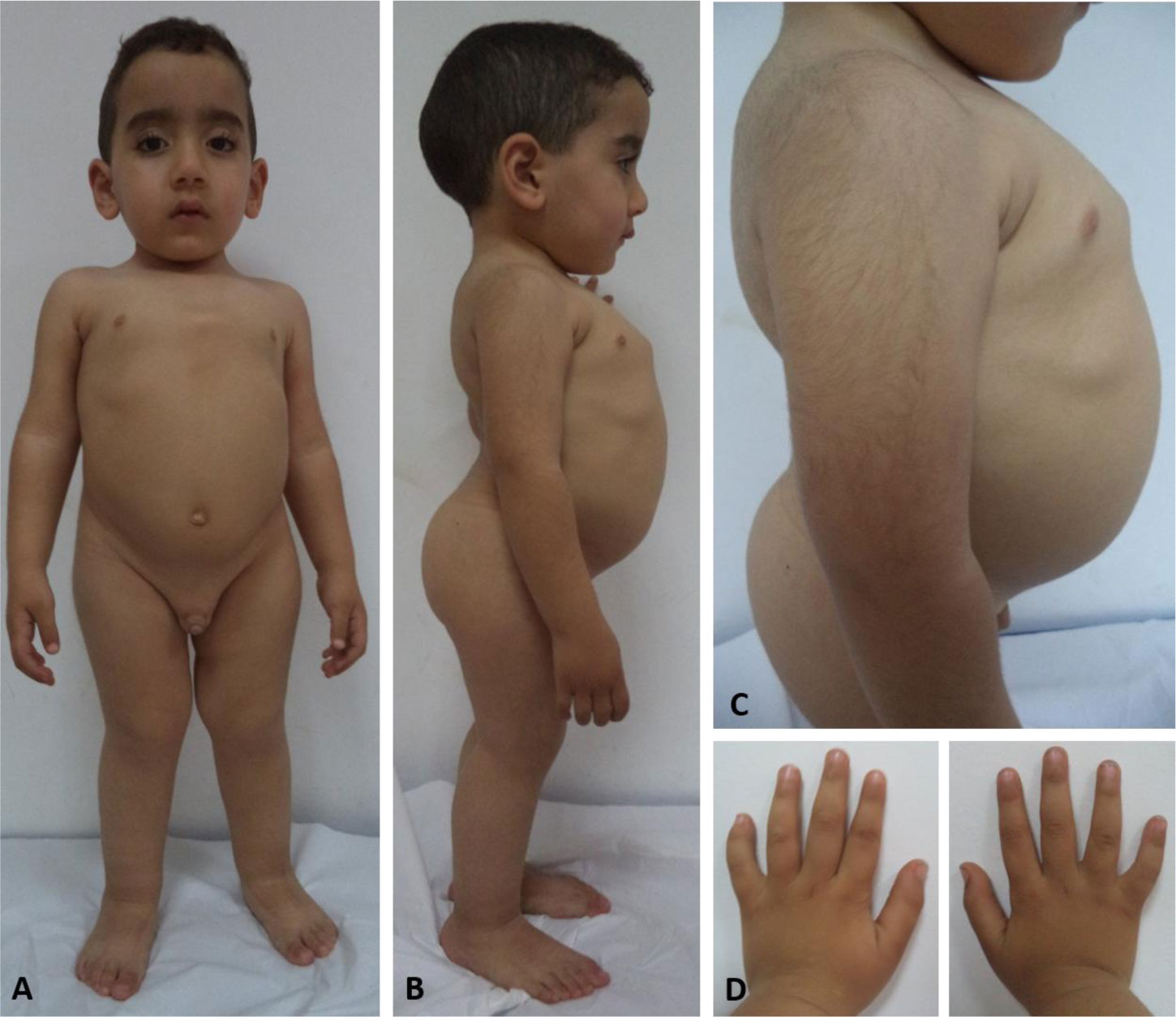
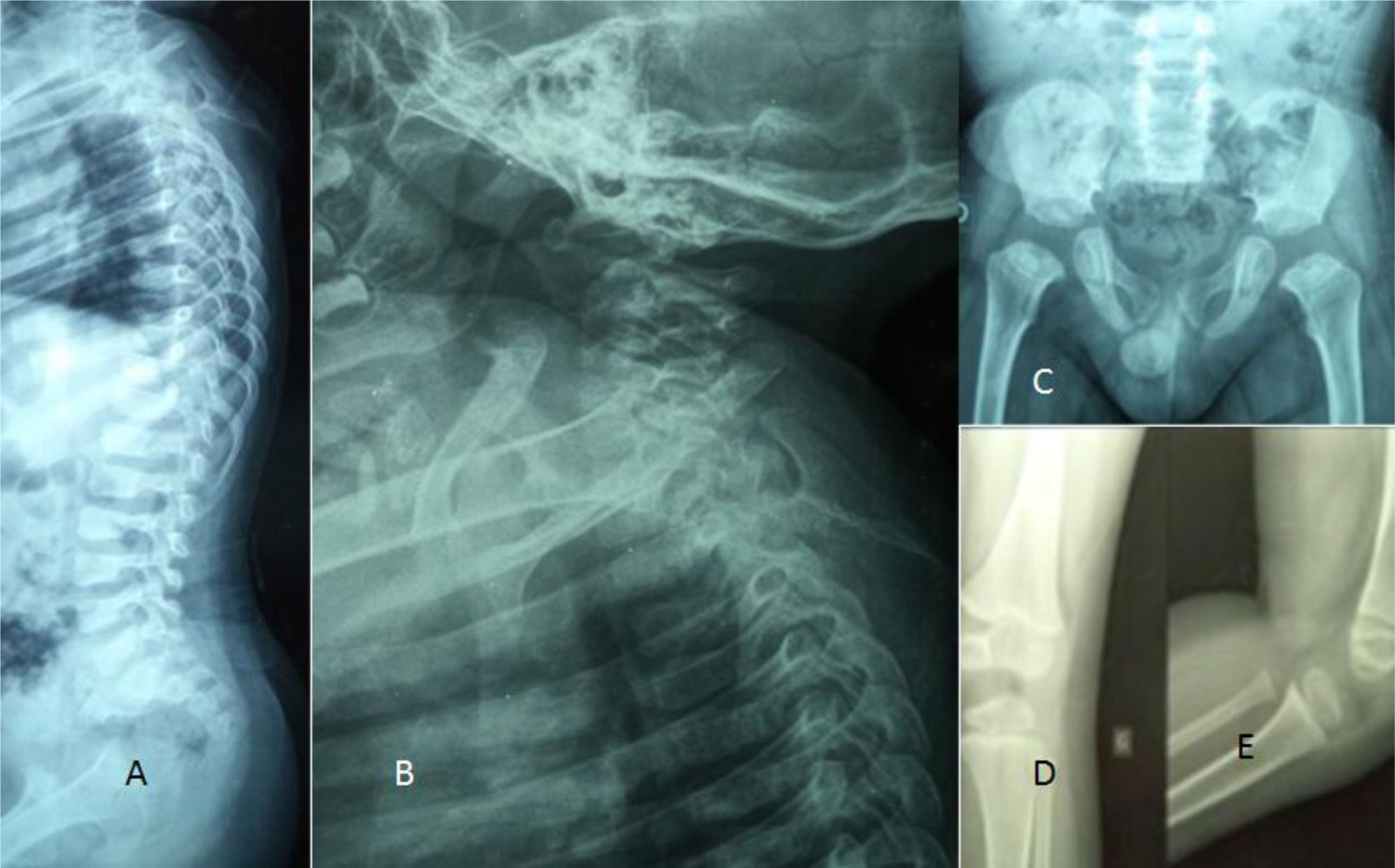
Osteochondrodysplasias are a heterogeneous group of genetic skeletal dysplasias. Mutations in the COL2A1 gene cause a spectrum of rare autosomal-dominant type II collagenopathies characterized by skeletal dysplasia, short stature, and with vision and auditory defects. In this study, we have investigated in more detail the phenotypic and genotypic characterization resulting from glycine to serine mutations in the COL2A1 gene in a 2-year-old boy.
Detailed clinical and radiological phenotypic characterization was the baseline tool to guide the geneticists toward proper genotypic confirmation.
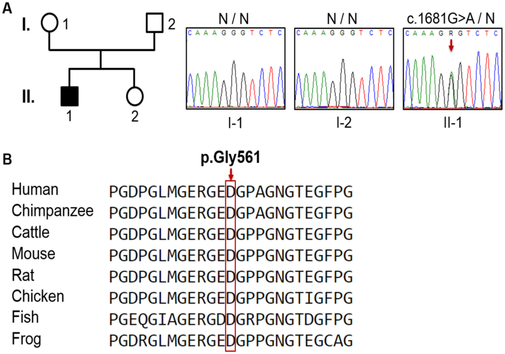
Genetic analysis revealed a de novo mutation, c.1681G>A (p.Gly561Ser), in the collagen type II alpha-1 gene (COL2A1). The identified variant showed impaired protein stability, and lead to dysfunction of type II collagen. In addition to pre and postnatal growth retardation, remarkable retardation of gross motor development and intellectual disability were noted. The latter was connected to cerebral malformations. The overall clinical phenotype of our current patient resembles spondyloepiphyseal dysplasia congenita (SEDC), but with extra phenotypic criteria.
The aim of this paper is twofold; firstly, raising awareness among orthopaedic surgeons when dealing with children manifesting multiple deformities, and secondly to broaden the clinical phenotype in patients with COL2A1 mutations of amino acid substitution (glycine to serine).
Citation: Mohammad Shboul, Hela Sassi, Houweyda Jilani, Imen Rejeb, Yasmina Elaribi, Syrine Hizem, Lamia Ben Jemaa, Marwa Hilmi, Susanna Gerit Kircher, Ali Al Kaissi. The phenotypic spectrum in a patient with Glycine to Serine mutation in the COL2A1 gene: overview study[J]. AIMS Molecular Science, 2021, 8(1): 76-85. doi: 10.3934/molsci.2021006
Osteochondrodysplasias are a heterogeneous group of genetic skeletal dysplasias. Mutations in the COL2A1 gene cause a spectrum of rare autosomal-dominant type II collagenopathies characterized by skeletal dysplasia, short stature, and with vision and auditory defects. In this study, we have investigated in more detail the phenotypic and genotypic characterization resulting from glycine to serine mutations in the COL2A1 gene in a 2-year-old boy.
Detailed clinical and radiological phenotypic characterization was the baseline tool to guide the geneticists toward proper genotypic confirmation.
Genetic analysis revealed a de novo mutation, c.1681G>A (p.Gly561Ser), in the collagen type II alpha-1 gene (COL2A1). The identified variant showed impaired protein stability, and lead to dysfunction of type II collagen. In addition to pre and postnatal growth retardation, remarkable retardation of gross motor development and intellectual disability were noted. The latter was connected to cerebral malformations. The overall clinical phenotype of our current patient resembles spondyloepiphyseal dysplasia congenita (SEDC), but with extra phenotypic criteria.
The aim of this paper is twofold; firstly, raising awareness among orthopaedic surgeons when dealing with children manifesting multiple deformities, and secondly to broaden the clinical phenotype in patients with COL2A1 mutations of amino acid substitution (glycine to serine).

| [1] |
Kannu P, Bateman J, Savarirayan R (2012) Clinical phenotypes associated with type II collagen mutations. J Paediatr Child Health 48: E38-43. doi: 10.1111/j.1440-1754.2010.01979.x

|
| [2] | Spranger J, Winterpacht A, Zabel B (1994) The type II collagenopathies: A spectrum of chondrodysplasias. Eur J Pediatr 153: 56-65. |
| [3] |
Cao LH, Wang L, Ji CY, et al. (2012) Novel and recurrent COL2A1 mutations in Chinese patients with spondyloepiphyseal dysplasia. Genet Mol Res 11: 4130-4137. doi: 10.4238/2012.September.27.1
|
| [4] |
Deng H, Huang X, Yuan L (2016) Molecular genetics of the COL2A1-related disorders. Mutat Res Rev Mutat Res 768: 1-13. doi: 10.1016/j.mrrev.2016.02.003
|
| [5] |
Nenna R, Turchetti A, Mastrogiorgio G, et al. (2019) COL2A1 gene mutations: Mechanisms of spondyloepiphyseal dysplasia congenita. Appl Clin Genet 12: 235-238. doi: 10.2147/TACG.S197205
|
| [6] |
Nishimura G, Haga N, Kitoh H, et al. (2005) The phenotypic spectrum of COL2A1 mutations. Hum Mutat 26: 36-43. doi: 10.1002/humu.20179
|
| [7] |
Barat-Houari M, Sarrabay G, Gatinois V, et al. (2016) Mutation Update for COL2A1 Gene Variants Associated with Type II Collagenopathies. Hum Mutat 37: 7-15. doi: 10.1002/humu.22915
|
| [8] |
Rukavina I, Mortier G, Van Laer L, et al. (2014) Mutation in the type II collagen gene (COL2AI) as a cause of primary osteoarthritis associated with mild spondyloepiphyseal involvement. Semin Arthritis Rheum 44: 101-104. doi: 10.1016/j.semarthrit.2014.03.003
|
| [9] |
Nazme NI, Sultana J, Chowdhury RB (2016) Escobar Syndrome - A Case Report in A Newborn. Bangladesh J Child Heal 39: 50-53. doi: 10.3329/bjch.v39i1.28359
|
| [10] | Exome Variant Server, NHLBI, 2014 Available from: https://evs.gs.washington.edu/EVS/. |
| [11] | Tafakhori A, Yu Jin Ng A, Tohari S, et al. (2016) Mutation in twinkle in a large Iranian family with progressive external ophthalmoplegia, myopathy, dysphagia and dysphonia, and behavior change. Arch Iran Med 19: 87-91. |
| [12] |
Zhang X, Minikel EV, O'Donnell-Luriaa AH, et al. (2017) ClinVar data parsing. Wellcome Open Res 2: 33. doi: 10.12688/wellcomeopenres.11640.1
|
| [13] |
Fokkema IFAC, Taschner PEM, Schaafsma GCP, et al. (2011) LOVD v.2.0: The next generation in gene variant databases. Hum Mutat 32: 557-563. doi: 10.1002/humu.21438
|
| [14] |
Karczewski KJ, Francioli LC, Tiao G, et al. (2020) The mutational constraint spectrum quantified from variation in 141,456 humans. Nature 581: 434-443. doi: 10.1038/s41586-020-2308-7
|
| [15] |
Lek M, Karczewski KJ, Minikel EV, et al. (2016) Analysis of protein-coding genetic variation in 60,706 humans. Nature 536: 285-291. doi: 10.1038/nature19057
|
| [16] |
Karczewski KJ, Weisburd B, Thomas B, et al. (2017) The ExAC browser: Displaying reference data information from over 60 000 exomes. Nucleic Acids Res 45: D840-845. doi: 10.1093/nar/gkw971
|
| [17] |
Richards S, Aziz N, Bale S, et al. (2015) Standards and guidelines for the interpretation of sequence variants: A joint consensus recommendation of the American College of Medical Genetics and Genomics and the Association for Molecular Pathology. Genet Med 17: 405-424. doi: 10.1038/gim.2015.30
|
| [18] |
Sim NL, Kumar P, Hu J, et al. (2012) SIFT web server: Predicting effects of amino acid substitutions on proteins. Nucleic Acids Res 40: W452-457. doi: 10.1093/nar/gks539
|
| [19] |
Adzhubei IA, Schmidt S, Peshkin L, et al. (2010) A method and server for predicting damaging missense mutations. Nat Methods 7: 248-249. doi: 10.1038/nmeth0410-248
|
| [20] |
Grantham R (1974) Amino acid difference formula to help explain protein evolution. Science 185: 862-864. doi: 10.1126/science.185.4154.862
|
| [21] |
Jagadeesh KA, Wenger AM, Berger MJ, et al. (2016) M-CAP eliminates a majority of variants of uncertain significance in clinical exomes at high sensitivity. Nat Genet 48: 1581-1586. doi: 10.1038/ng.3703
|
| [22] |
Pollard KS, Hubisz MJ, Rosenbloom KR, et al. (2010) Detection of nonneutral substitution rates on mammalian phylogenies. Genome Res 20: 110-121. doi: 10.1101/gr.097857.109
|
| [23] |
Schwarz JM, Cooper DN, Schuelke M, et al. (2014) Mutationtaster2: Mutation prediction for the deep-sequencing age. Nat Methods 11: 361-362. doi: 10.1038/nmeth.2890
|
| [24] |
Kõressaar T, Lepamets M, Kaplinski L, et al. (2018) Primer3-masker: Integrating masking of template sequence with primer design software. Bioinformatics 34: 1937-1938. doi: 10.1093/bioinformatics/bty036
|
| [25] |
Corpet F (1988) Multiple sequence alignment with hierarchical clustering. Nucleic Acids Res 16: 10881-10890. doi: 10.1093/nar/16.22.10881
|
| [26] |
Liu YF, Chen WM, Lin YF, et al. (2005) Type II Collagen Gene Variants and Inherited Osteonecrosis of the Femoral Head. N Engl J Med 352: 2294-2301. doi: 10.1056/NEJMoa042480
|
| [27] |
Barat-Houari M, Dumont B, Fabre A, et al. (2016) The expanding spectrum of COL2A1 gene variants in 136 patients with a skeletal dysplasia phenotype. Eur J Hum Genet 24: 992-1000. doi: 10.1038/ejhg.2015.250
|
| [28] |
Terhal PA, Nievelstein RJAJ, Verver EJJ, et al. (2015) A study of the clinical and radiological features in a cohort of 93 patients with a COL2A1 mutation causing spondyloepiphyseal dysplasia congenita or a related phenotype. Am J Med Genet Part A 167: 461-475. doi: 10.1002/ajmg.a.36922
|
| [29] |
Husar-Memmer E, Ekici A, Al Kaissi A, et al. (2013) Premature Osteoarthritis as Presenting Sign of Type II Collagenopathy: A Case Report and Literature Review. Semin Arthritis Rheum 42: 355-360. doi: 10.1016/j.semarthrit.2012.05.002
|
| [30] |
Al Kaissi A, Laccone F, Karner C, et al. (2013) Hip dysplasia and spinal osteochondritis (Scheuermann's disease) in a girl with type II manifesting collagenopathy. Orthopade 42: 963-968. doi: 10.1007/s00132-013-2182-1
|
| [31] |
Chen J, Ma X, Zhou Y, et al. (2017) Recurrent c.G1636A (p.G546S) mutation of COL2A1 in a Chinese family with skeletal dysplasia and different metaphyseal changes: a case report. BMC Pediatr 17: 175. doi: 10.1186/s12887-017-0930-9
|
| [32] |
Anderson CE, Sillence DO, Lachman RS, et al. (1982) Spondylometepiphyseal dysplasia, Strudwick type. Am J Med Genet 13: 243-256. doi: 10.1002/ajmg.1320130304
|
Figures(3) / Tables(3)

Mohammad Shboul, Hela Sassi, Houweyda Jilani, Imen Rejeb, Yasmina Elaribi, Syrine Hizem, Lamia Ben Jemaa, Marwa Hilmi, Susanna Gerit Kircher, Ali Al Kaissi. The phenotypic spectrum in a patient with Glycine to Serine mutation in the COL2A1 gene: overview study[J]. AIMS Molecular Science, 2021, 8(1): 76-85. doi: 10.3934/molsci.2021006


 DownLoad: