The paper presents an augmented curvilinear virtual element method to determine homogenized in-plane shear material moduli of long-fibre reinforced composites in the framework of asymptotic homogenization method. The new virtual element combine an exact representation of the curvilinear computational geometry for complex fibre cross section shapes through an innovative two-dimensional cubature suite for NURBS-like polygonal domains. A selection of representative numerical tests supports the accuracy and efficiency of the proposed approach for both doubly periodic and random fibre arrangement with matrix domain.
Citation: E. Artioli, G. Elefante, A. Sommariva, M. Vianello. Homogenization of composite materials reinforced with unidirectional fibres with complex curvilinear cross section: a virtual element approach[J]. Mathematics in Engineering, 2024, 6(4): 510-535. doi: 10.3934/mine.2024021
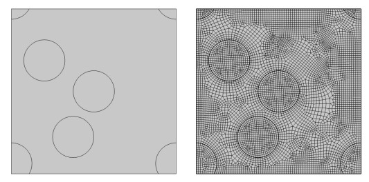
The paper presents an augmented curvilinear virtual element method to determine homogenized in-plane shear material moduli of long-fibre reinforced composites in the framework of asymptotic homogenization method. The new virtual element combine an exact representation of the curvilinear computational geometry for complex fibre cross section shapes through an innovative two-dimensional cubature suite for NURBS-like polygonal domains. A selection of representative numerical tests supports the accuracy and efficiency of the proposed approach for both doubly periodic and random fibre arrangement with matrix domain.

| [1] | T. M. Apostol, Calculus, 2 Eds., Vol. Ⅱ, Blaisdell, 1969. |
| [2] |
E. Artioli, Asymptotic homogenization of fibre-reinforced composites: a virtual element method approach, Meccanica, 53 (2018), 1187–1201. https://doi.org/10.1007/s11012-018-0818-2 doi: 10.1007/s11012-018-0818-2

|
| [3] |
E. Artioli, L. Beirão da Veiga, M. Verani, An adaptive curved virtual element method for the statistical homogenization of random fibre-reinforced composites, Finite Elem. Anal. Des., 177 (2020), 103418. https://doi.org/10.1016/j.finel.2020.103418 doi: 10.1016/j.finel.2020.103418
|
| [4] |
E. Artioli, A. Sommariva, M. Vianello, Algebraic cubature on polygonal elements with a circular edge, Comput. Math. Appl., 79 (2020), 2057–2066. https://doi.org/10.1016/j.camwa.2019.10.022 doi: 10.1016/j.camwa.2019.10.022
|
| [5] |
L. Beirão da Veiga, F. Brezzi, A. Cangiani, G. Manzini, L. D. Marini, A. Russo, Basic principles of virtual element methods, Math. Models Methods Appl. Sci., 23 (2013), 199–214. https://doi.org/10.1142/S0218202512500492 doi: 10.1142/S0218202512500492
|
| [6] |
L. Beirão da Veiga, F. Brezzi, L. D. Marini, A. Russo, The Hitchhiker's guide to the virtual element method, Math. Models Methods Appl. Sci., 24 (2014), 1541–1573. https://doi.org/10.1142/S021820251440003X doi: 10.1142/S021820251440003X
|
| [7] |
L. Beirão da Veiga, A. Russo, G. Vacca, The virtual element method with curved edges, ESAIM: M2AN, 53 (2019), 375–404. https://doi.org/10.1051/m2an/2018052 doi: 10.1051/m2an/2018052
|
| [8] |
L. Beirão da Veiga, F. Brezzi, L. D. Marini, A. Russo, Polynomial preserving virtual elements with curved edges, Math. Models Methods Appl. Sci., 30 (2020), 1555–1590. https://doi.org/10.1142/S0218202520500311 doi: 10.1142/S0218202520500311
|
| [9] | A. Bensoussan, J. Lions, G. Papanicolau, Asymptotic analysis for periodic structures, Studies in Mathematics and Its Applications, Vol. 5, North-Holland, 1978. |
| [10] |
D. Bigoni, S. K. Serkov, M. Valentini, A. B. Movchan, Asymptotic models of dilute composites with imperfectly bonded inclusions, Int. J. Solids Struct., 35 (1998), 3239–3258. https://doi.org/10.1016/S0020-7683(97)00366-1 doi: 10.1016/S0020-7683(97)00366-1
|
| [11] |
P. J. Davis, A construction of nonnegative approximate quadratures, Math. Compt., 21 (1967), 578–582. https://doi.org/10.2307/2005001 doi: 10.2307/2005001
|
| [12] | C. de Boor, A practical guide to splines, Springer-Verlag, 1978. |
| [13] |
K. Deckers, A. Mougaida, H. Belhadjsalah, Algorithm 973: extended rational Fejér quadrature rules based on Chebyshev orthogonal rational functions, ACM Trans. Math. Software, 43 (2017), 1–29. https://doi.org/10.1145/3054077 doi: 10.1145/3054077
|
| [14] |
M. Dessole, M. Dell'Orto, F. Marcuzzi, The Lawson‐Hanson algorithm with deviation maximization: finite convergence and sparse recovery, Numer. Linear Algebra Appl., 30 (2023), e2490. https://doi.org/10.1002/nla.2490 doi: 10.1002/nla.2490
|
| [15] |
M. Dessole, F. Marcuzzi, M. Vianello, dCATCH–A numerical package for d-variate near G-optimal Tchakaloff regression via fast NNLS, Mathematics, 8 (2020), 1122. https://doi.org/10.3390/math8071122 doi: 10.3390/math8071122
|
| [16] |
M. Dessole, F. Marcuzzi, M. Vianello, Accelerating the Lawson-Hanson NNLS solver for large-scale Tchakaloff regression designs, Dolomites Res. Notes Approx., 13 (2020), 20–29. https://doi.org/10.14658/PUPJ-DRNA-2020-1-3 doi: 10.14658/PUPJ-DRNA-2020-1-3
|
| [17] |
T. Kanit, S. Forest, I. Galliet, V. Mounoury, D. Jeulin, Determination of the size of the representative volume element for random composites: statistical and numerical approach, Int. J. Solids Struct., 40 (2003), 3467–3679. https://doi.org/10.1016/S0020-7683(03)00143-4 doi: 10.1016/S0020-7683(03)00143-4
|
| [18] |
N. Hale, A. Townsend, Fast and accurate computation of Gauss-Legendre and Gauss-Jacobi quadrature nodes and weights, SIAM J. Sci. Comput., 35 (2013), A652–A674. https://doi.org/10.1137/120889873 doi: 10.1137/120889873
|
| [19] |
Z. Hashin, The spherical inclusion with imperfect interface, J. Appl. Mech., 58 (1991), 444–449. https://doi.org/10.1115/1.2897205 doi: 10.1115/1.2897205
|
| [20] | C. L. Lawson, R. J. Hanson, Solving least squares problems, Classics in Applied Mathematics, SIAM, 1995. |
| [21] |
F. Lene, D. Leguillon, Homogenized constitutive law for a partially cohesive composite material, Int. J. Solids Struct., 18 (1982), 443–458. https://doi.org/10.1016/0020-7683(82)90082-8 doi: 10.1016/0020-7683(82)90082-8
|
| [22] |
L. Mascotto, The role of stabilization in the virtual element method: a survey, Comput. Math. Appl., 151 (2023), 244–251. https://doi.org/10.1016/j.camwa.2023.09.045 doi: 10.1016/j.camwa.2023.09.045
|
| [23] |
M. Ostoja-Starzewski, Material spatial randomness: from statistical to representative volume element, Probab. Eng. Mech., 21 (2006), 112–132. https://doi.org/10.1016/j.probengmech.2005.07.007 doi: 10.1016/j.probengmech.2005.07.007
|
| [24] | L. Piegl, W. Tiller, The NURBS book, 2 Eds., Springer-Verlag, 1997. |
| [25] | E. Sanchez-Palencia, Non-homogeneous media and vibration theory, Lecture Notes in Physics, Springer, 1980. https://doi.org/10.1007/3-540-10000-8 |
| [26] |
R. Sevilla, S. Fernández-Méndez, Numerical integration over 2D NURBS-shaped domains with applications to NURBS-enhanced FEM, Finite Elem. Anal. Des., 47 (2011), 1209–1220. https://doi.org/10.1016/j.finel.2011.05.011 doi: 10.1016/j.finel.2011.05.011
|
| [27] | M. Slawski, Non-negative least squares: comparison of algorithms. Available from: https://sites.google.com/site/slawskimartin/code. |
| [28] | A. Sommariva, Indomain routines for NURBS, composite Bezier or bivariate parametric splines domains, alvisesommariva/inRS. Available from: https://github.com/alvisesommariva/inRS. |
| [29] | A. Sommariva, Software for computing algebraic cubature rules of degree n on domains defined parametrically by rational splines, alvisesommariva/CUB_RS. Available from: https://github.com/alvisesommariva/CUB_RS. |
| [30] |
A. Sommariva, M. Vianello, inRS: Implementing the indicator function of NURBS-shaped planar domains, Appl. Math. Lett., 130 (2022), 108026. https://doi.org/10.1016/j.aml.2022.108026 doi: 10.1016/j.aml.2022.108026
|
| [31] |
A. Sommariva, M. Vianello, Low cardinality Positive Interior cubature on NURBS-shaped domains, Bit Numer. Math., 63 (2023), 22. https://doi.org/10.1007/s10543-023-00958-y doi: 10.1007/s10543-023-00958-y
|
| [32] | A. Sommariva, M. Vianello, Computing Tchakaloff-like cubature rules on spline curvilinear polygons, Dolomit. Res. Notes Approximation, 14 (2021), 1–11. |
| [33] | V. Tchakaloff, Formules de cubatures mécaniques à coefficients non négatifs, Bull. Sci. Math., 81 (1957), 123–134. |
| [34] |
D. R. Wilhelmsen, A nearest point algorithm for convex polyhedral cones and applications to positive linear approximation, Math. Comp., 30 (1976), 48–57. https://doi.org/10.1090/S0025-5718-1976-0394439-5 doi: 10.1090/S0025-5718-1976-0394439-5
|
| [35] |
D. Gunderman, K. Weiss, J. A. Evans, Spectral mesh-free quadrature for planar regions bounded by rational parametric curves, Comput.-Aided Des., 130 (2021), 102944. https://doi.org/10.1016/j.cad.2020.102944 doi: 10.1016/j.cad.2020.102944
|
| [36] |
A. Sommariva, M. Vianello, Compression of multivariate discrete measures and applications, Numer. Funct. Anal. Optim., 36 (2015), 1198–1223. https://doi.org/10.1080/01630563.2015.1062394 doi: 10.1080/01630563.2015.1062394
|


Figures(16) / Tables(1)

E. Artioli, G. Elefante, A. Sommariva, M. Vianello. Homogenization of composite materials reinforced with unidirectional fibres with complex curvilinear cross section: a virtual element approach[J]. Mathematics in Engineering, 2024, 6(4): 510-535. doi: 10.3934/mine.2024021


 DownLoad: