Microtubule gliding assays have been an important experimental tool for investigating intracellular molecular motor transport systems. A statistical method to estimate the parameters of a stochastic model describing the movement of a microtubule in a kinesin-microtubule gliding assay experiment is presented. Two models are proposed: the first is an approximate discretization and modification of an existing system of stochastic differential equations describing microtubule motion proposed by Gibbons et al. (2001), and a second version accommodates some behaviors encountered in motility assay experiments, such as curvature and pausing. To aid in understanding the relationship between kinesin motors and microtubules, the model describes metrics such as the velocity of a microtubule in a gliding assay experiment, the effect on the velocity based on the amount of curvature in the microtubule, and how frequently a microtubule may pause its movement. Parameter estimation for the models will employ a stochastic expectation-maximization (EM) algorithm with the expectation step approximated by particle filtering techniques.
Citation: John Stockton, John Fricks. State-space modeling and estimation for motility assay experiments[J]. Mathematical Biosciences and Engineering, 2026, 23(11): 3320-3347. doi: 10.3934/mbe.2026114
Microtubule gliding assays have been an important experimental tool for investigating intracellular molecular motor transport systems. A statistical method to estimate the parameters of a stochastic model describing the movement of a microtubule in a kinesin-microtubule gliding assay experiment is presented. Two models are proposed: the first is an approximate discretization and modification of an existing system of stochastic differential equations describing microtubule motion proposed by Gibbons et al. (2001), and a second version accommodates some behaviors encountered in motility assay experiments, such as curvature and pausing. To aid in understanding the relationship between kinesin motors and microtubules, the model describes metrics such as the velocity of a microtubule in a gliding assay experiment, the effect on the velocity based on the amount of curvature in the microtubule, and how frequently a microtubule may pause its movement. Parameter estimation for the models will employ a stochastic expectation-maximization (EM) algorithm with the expectation step approximated by particle filtering techniques.

| [1] |
R. D. Vale, T. S. Reese, M. P. Sheetz, Identification of a novel force-generating protein, kinesin, involved in microtubule-based motility, Cell, 42 (1985), 39–50. https://doi.org/10.1016/S0092-8674(85)80099-4 doi: 10.1016/S0092-8674(85)80099-4
|
| [2] |
J. Howard, A. J. Hudspeth, R. D. Vale, Movement of microtubules by single kinesin molecules, Nature, 342 (1989), 154–158. https://doi.org/10.1038/342154a0 doi: 10.1038/342154a0
|
| [3] |
C. V. Sindelar, K. H. Downing. The beginning of kinesin's force-generating cycle visualized at 9-Å resolution, J. Cell Biol., 177 (2007), 377–385. https://doi.org/10.1083/jcb.200612090 doi: 10.1083/jcb.200612090
|
| [4] |
N. Hirokawa, K. K. Pfister, H. Yorifuji, M. C. Wagner, S. T. Brady, G. S. Bloom, Submolecular domains of bovine brain kinesin identified by electron microscopy and monoclonal antibody decoration, Cell, 56 (1989), 867–878. https://doi.org/10.1016/0092-8674(89)90691-0 doi: 10.1016/0092-8674(89)90691-0
|
| [5] |
A. Yildiz, M. Tomishige, R. D. Vale, P. R. Selvin, Kinesin walks hand-over-hand, Science, 303 (2004), 676–678. https://doi.org/10.1126/science.1093753 doi: 10.1126/science.1093753
|
| [6] |
S. E. Rice, A. W. Lin, D. Safer, C. L. Hart, N. I. Naber, B. Carragher, et al., A structural change in the kinesin motor protein that drives motility, Nature, 402 (1999), 778–784. https://doi.org/10.1038/45483 doi: 10.1038/45483
|
| [7] |
S. L. Rogers, J. M. Scholey, Motility assays for microtubule motor proteins, Encycl. Life Sci., 2004 (2004). https://doi.org/10.1038/npg.els.0002621 |
| [8] |
W. O. Hancock, J. Howard, Processivity of the motor protein kinesin requires two heads, J. Cell Biol., 140 (1998), 1395–1405. https://doi.org/10.1083/jcb.140.6.1395 doi: 10.1083/jcb.140.6.1395
|
| [9] |
G. Arpağ, S. Shastry, W. O. Hancock, E. Tüzel, Transport by populations of fast and slow kinesins uncovers novel family-dependent motor characteristics important for in vivo function, Biophys. J., 107 (2014), 1896–1904. https://doi.org/10.1016/j.bpj.2014.09.009 doi: 10.1016/j.bpj.2014.09.009
|
| [10] |
R. Grover, J. Fischer, F. W. Schwarz, W. J. Walter, P. Schwille, S. Diez, Transport efficiency of membrane-anchored kinesin-1 motors depends on motor density and diffusivity, Proc. Natl. Acad. Sci., 113 (2016), E7185–E7193. https://doi.org/10.1073/pnas.1611398113 doi: 10.1073/pnas.1611398113
|
| [11] |
R. Jiang, S. Vandal, S. Park, S. Majd, E. Tüzel, W. O. Hancock, Microtubule binding kinetics of membrane-bound kinesin-1 predicts high motor copy numbers on intracellular cargo, Proc. Natl. Acad. Sci. U.S.A., 116 (2019), 26564–26570. https://doi.org/10.1073/pnas.1916204116 doi: 10.1073/pnas.1916204116
|
| [12] |
F. Gibbons, J. Chauwin, M. Despósito, J. V. José, A dynamical model of kinesin-microtubule motility assays, Biophys. J., 80 (2001), 2515–2526. https://doi.org/10.1016/S0006-3495(01)76223-6 doi: 10.1016/S0006-3495(01)76223-6
|
| [13] |
A. Doucet, N. de Freitas, N. Gordon, An introduction to sequential monte carlo methods, in Sequential Monte Carlo Methods in Practice, Springer, (2001), 3–14. https://doi.org/10.1007/978-1-4757-3437-9_1 |
Figures(15) / Tables(2)

John Stockton, John Fricks. State-space modeling and estimation for motility assay experiments[J]. Mathematical Biosciences and Engineering, 2026, 23(11): 3320-3347. doi: 10.3934/mbe.2026114

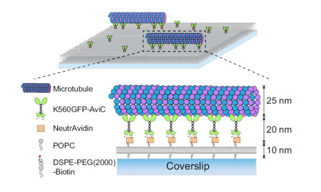
Diagram modeling a microtubule gliding assay experiment on a glass coverslip. K560GFP-AviC refers to biotinylated GFP-labeled Drosophila kinesin-1 motors, NeutrAvidin is the link to DSPE-PEG(2000)-Biotin. This diagram depicts a lipid bilayer composed of POPC (1-palmitoyl-2-oleoyl-glycero-3-phosphocholine) that is not present in the experimental data used in this document. (Image Source: [11])
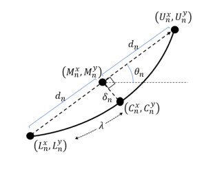
Visual diagram of the microtubule with its model notation. The solid black curve represents the microtubule itself, where $ \lambda $ represents the arc length of the entire microtubule
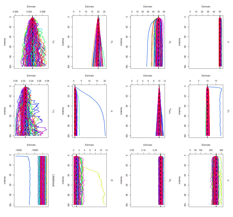
The results of 100 simulations generated under the framework of the full model, each having 100 iterations of the EM algorithm performed. The true values used to simulate each series are shown in the dashed black line. In this experiment, the EM algorithm was provided an initial value for each parameter equal to the true value of the parameter used to generate the simulations. The plot in the lower right corner depicts a stochastic approximation of the likelihood
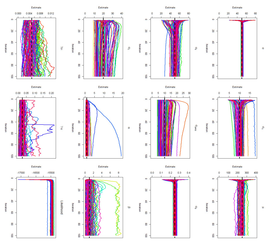
The results of 100 simulations generated under the framework of the full model, each having 100 iterations of the EM algorithm performed. The true values used to simulate each series are shown in the dotted black line. In this experiment, the EM algorithm was provided an initial value for each parameter that was generated from a uniform distributed with a lower bound that was $ 0.4 \theta_0 $ and an upper bound of $ 1.6 \theta_0 $, where $ \theta_0 $ is the true value of the parameter used for generating the simulations. The plot in the lower right corner depicts a stochastic approximation of the likelihood
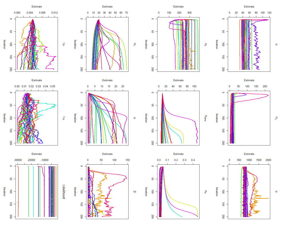
The results of 200 iterations of the stochastic EM algorithm for the 28 series of experimental data across the 11 parameters using the full version of the model as well as a stochastic estimate of the log-likelihood. Matching colors across each of the graphs designate the same series
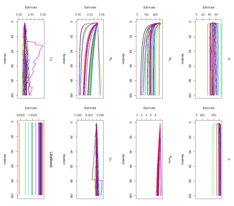
The results of 200 iterations of the stochastic EM algorithm for the 28 series of experimental data across the seven parameters remaining after removing any aspect related to microtubule bending to form the reduced version of the model. The stochastic estimate of the log-likelihood is also included. Matching colors across each of the graphs designate the same series
For a series simulated as the full model, this plot depicts the residuals from using the full model as the method of parameter estimation
For a series simulated as the full model, this plot depicts the residuals from using the reduced model as the method of parameter estimation
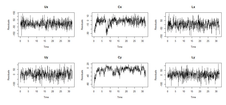
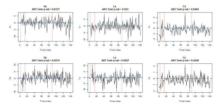
The standardized residuals for each of the six variables considered in the observation equations for the full version of the model
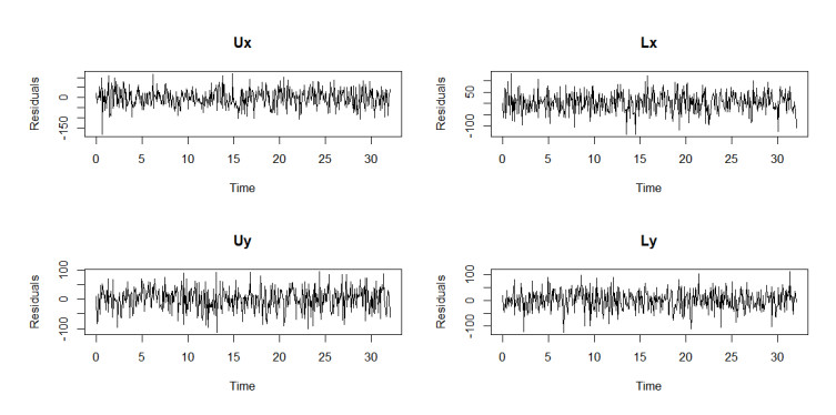
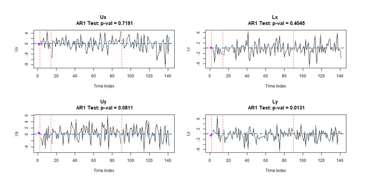
The standardized residuals for each of the four variables considered in the observation equations for the reduced version of the model
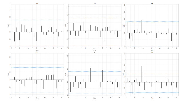
PACF plots for each of the six variables considered in the observation equations for the full version of the model
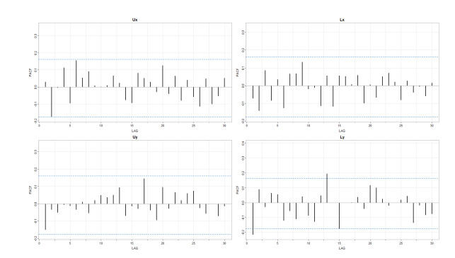
PACF plots for each of the four variables considered in the observation equations for the reduced version of the model
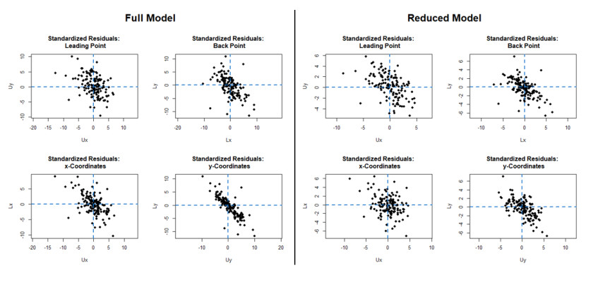
Residual comparison for the full version of the model comprises the 2 $ \times $ 2 grid of plots on the left. The 2 $ \times $ 2 grid of plots on the right correspond to the results using the reduced version of the model for the same series
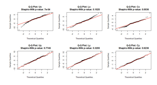
Normal probability plots for the standardized residuals for all six variables in the observation equations in the full version of the model
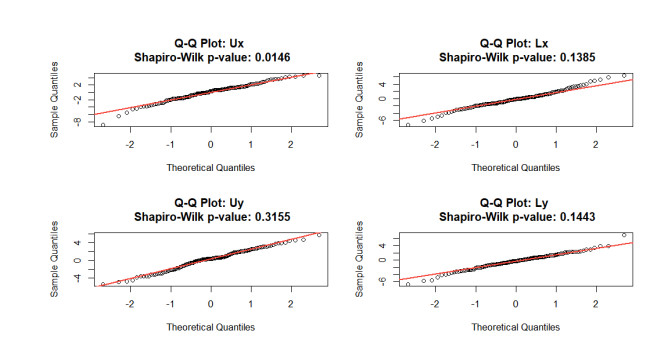
Normal probability plots for the standardized residuals for all four variables in the observation equations in the reduced version of the model




 DownLoad: