Global dynamics of a discrete two-population model for flour beetle growth

Samantha J. Brozak; Kamrun N. Keya; Denise Dengi; Sophia Peralta; John D. Nagy; Yang Kuang; Samantha J. Brozak; Kamrun N. Keya; Denise Dengi; Sophia Peralta; John D. Nagy; Yang Kuang

doi:10.3934/mbe.2025072

Mathematical Biosciences and Engineering

2025, Volume 22, Issue 8: 1980-1998. doi: 10.3934/mbe.2025072

Previous Article Next Article

Research article

Global dynamics of a discrete two-population model for flour beetle growth

1.
School of Mathematical and Statistical Sciences, Arizona State University, Tempe 85287, USA
2.
Department of Mathematics, University of California Berkeley, Berkeley 94720, USA
3.
Department of Life Sciences, Scottsdale Community College, Scottsdale 85256, USA

^† These authors contributed equally.
Academic Editor: Gail Wolkowicz

Received: 29 April 2025 Revised: 27 May 2025 Accepted: 09 June 2025 Published: 25 June 2025

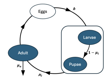
The cannibalistic behavior of Tribolium has been extensively researched, revealing instances of chaotic dynamics in laboratory environments for Tribolium castaneum. The well-established Larvae-Pupae-Adult (LPA) model has been instrumental in understanding the conditions that lead to chaos in flour beetles (genus: Tribolium). In response to new experimental observations showing a decline in the pupae population in Tribolium confusum, we proposed and analyzed a simplified two-stage Larvae-Adult (LA) model. This model integrated the pupae population within the larval group, similar to that of the original LPA model, with development transitions governed by internal rates. By applying the model to time-series data, we demonstrated its effectiveness in capturing short-term population fluctuations in T. confusum. We established the model's positivity and boundedness, perform stability analyses of both trivial and positive steady states, and explored bifurcations and steady-state behavior through numerical simulations. We proved global stability for the extinction and positive steady states and observed additional restrictions required for stability compared to the LPA model. Our results indicated that while chaos was a possible outcome, it was infrequent within the practical parameter ranges observed, with environmental changes related to media and nutrient alterations being more likely triggers.
- flour beetles,
- discrete map,
- matrix model,
- LPA model,
- Tribolium,
- population model
Citation: Samantha J. Brozak, Kamrun N. Keya, Denise Dengi, Sophia Peralta, John D. Nagy, Yang Kuang. Global dynamics of a discrete two-population model for flour beetle growth[J]. Mathematical Biosciences and Engineering, 2025, 22(8): 1980-1998. doi: 10.3934/mbe.2025072

Related Papers:

Abstract

The cannibalistic behavior of Tribolium has been extensively researched, revealing instances of chaotic dynamics in laboratory environments for Tribolium castaneum. The well-established Larvae-Pupae-Adult (LPA) model has been instrumental in understanding the conditions that lead to chaos in flour beetles (genus: Tribolium). In response to new experimental observations showing a decline in the pupae population in Tribolium confusum, we proposed and analyzed a simplified two-stage Larvae-Adult (LA) model. This model integrated the pupae population within the larval group, similar to that of the original LPA model, with development transitions governed by internal rates. By applying the model to time-series data, we demonstrated its effectiveness in capturing short-term population fluctuations in T. confusum. We established the model's positivity and boundedness, perform stability analyses of both trivial and positive steady states, and explored bifurcations and steady-state behavior through numerical simulations. We proved global stability for the extinction and positive steady states and observed additional restrictions required for stability compared to the LPA model. Our results indicated that while chaos was a possible outcome, it was infrequent within the practical parameter ranges observed, with environmental changes related to media and nutrient alterations being more likely triggers.

References

[1]	M. D. Pointer, M. J. G. Gage, L. G. Spurgin, Tribolium beetles as a model system in evolution and ecology, Heredity, 126 (2021), 869–883. https://doi.org/10.1038/s41437-021-00420-1 doi: 10.1038/s41437-021-00420-1
[2]	R. F. Costantino, J. M. Cushing, B. Dennis, R. A. Desharnais, Experimentally induced transitions in the dynamic behaviour of insect populations, Nature, 375 (1995), 227–230. https://doi.org/10.1038/375227a0 doi: 10.1038/375227a0
[3]	R. F. Costantino, R. A. Desharnais, J. M. Cushing, B. Dennis, Chaotic dynamics in an insect population, Science, 275 (1997), 389–391. https://doi.org/10.1126/science.275.5298.389 doi: 10.1126/science.275.5298.389
[4]	T. Park, Interspecies competition in populations of Tribolium confusum Duval and Tribolium castaneum Herbst, Ecol. Monogr., 18 (1948), 265–307. https://doi.org/10.2307/1948641 doi: 10.2307/1948641
[5]	T. Park, Experimental studies of interspecies competition Ⅱ. temperature, humidity, and competition in two species of Tribolium, Physiol. Zool., 27 (1954), 177–238. https://doi.org/10.1086/physzool.27.3.30152164 doi: 10.1086/physzool.27.3.30152164
[6]	T. Park, Experimental studies of interspecies competition. Ⅲ relation of initial species proportion to competitive outcome in populations of Tribolium, Physiol. Zool., 30 (1957), 22–40. https://doi.org/10.1086/physzool.30.1.30166306 doi: 10.1086/physzool.30.1.30166306
[7]	M. S. Bartlett, On theoretical models for competitive and predatory biological systems, Biometrika, 44 (1957), 27–42. https://doi.org/10.2307/2333238 doi: 10.2307/2333238
[8]	R. M. May, Biological populations with nonoverlapping generations: Stable points, stable cycles, and chaos, Science, 186 (1974), 645–647. https://doi.org/10.1126/science.186.4164.645 doi: 10.1126/science.186.4164.645
[9]	B. Dennis, R. A. Desharnais, J. M. Cushing, S. M. Henson, R. F. Costantino, Estimating chaos and complex dynamics in an insect population, Ecol. Monogr., 71 (2001), 277–303. https://doi.org/10.1890/0012-9615(2001)071[0277:ECACDI]2.0.CO;2 doi: 10.1890/0012-9615(2001)071[0277:ECACDI]2.0.CO;2
[10]	S. J. Brozak, S. Peralta, T. Phan, J. D. Nagy, Y. Kuang, Dynamics of an LPAA model for Tribolium growth: Insights into population chaos, SIAM J. Appl. Math., 84 (2024), 2300–2320. https://doi.org/10.1137/24M1633881 doi: 10.1137/24M1633881
[11]	H. P. Benoît, E. McCauley, J. R. Post, Testing the demographic consequences of cannibalism in Tribolium confusum, Ecology, 79 (1998), 2839–2851. https://doi.org/10.1890/0012-9658(1998)079[2839:TTDCOC]2.0.CO;2 doi: 10.1890/0012-9658(1998)079[2839:TTDCOC]2.0.CO;2
[12]	T. Park, D. B. Mertz, M. Nathanson, The cannibalism of pupae by adult flour Beetles, Physiol. Zool., 41 (1968), 228–253. https://doi.org/10.1086/physzool.41.2.30155454 doi: 10.1086/physzool.41.2.30155454
[13]	A. Veprauskas, J. M. Cushing, A juvenile–adult population model: Climate change, cannibalism, reproductive synchrony, and strong Allee effects, J. Biol. Dyn., 11 (2017), 1–24. https://doi.org/10.1080/17513758.2015.1131853 doi: 10.1080/17513758.2015.1131853
[14]	S. Via, Cannibalism facilitates the use of a novel environment in the flour beetle, Tribolium castaneum, Heredity, 82 (1999), 267–275. https://doi.org/10.1038/sj.hdy.6884820 doi: 10.1038/sj.hdy.6884820
[15]	J. Cushing, Systems of difference equations and structured population dynamics, in Proceedings of the First International Conference on Difference Equations, (1994), 123–132.
[16]	S. M. Henson, R. F. Costantino, R. A. Desharnais, J. M. Cushing, B. Dennis, Basins of attraction: Population dynamics with two stable 4-cycles, Oikos, 98 (2002), 17–24. https://doi.org/10.1034/j.1600-0706.2002.980102.x doi: 10.1034/j.1600-0706.2002.980102.x
[17]	S. M. Henson, J. M. Cushing, The effect of periodic habitat fluctuations on a nonlinear insect population model, J. Math. Biol., 36 (1997), 201–226, https://doi.org/10.1007/s002850050098 doi: 10.1007/s002850050098
[18]	S. M. Henson, J. M. Cushing, R. F. Costantino, B. Dennis, R. A. Desharnais, Phase switching in population cycles, Proc. R. Soc. London, Ser. B: Biol. Sci., 265 (1998), 2229–2234. https://doi.org/10.1098/rspb.1998.0564 doi: 10.1098/rspb.1998.0564
[19]	S. M. Henson, R. F. Costantino, J. M. Cushing, B. Dennis, R. A. Desharnais, Multiple attractors, saddles, and population dynamics in periodic habitats, Bull. Math. Biol., 61 (1999), 1121–1149. https://doi.org/10.1006/bulm.1999.0136 doi: 10.1006/bulm.1999.0136
[20]	S. M. Henson, Multiple attractors and resonance in periodically forced population models, Physica D: Nonlinear Phenom., 140 (2000), 33–49. https://doi.org/10.1016/S0167-2789(99)00231-6 doi: 10.1016/S0167-2789(99)00231-6
[21]	S. M. Henson, R. F. Costantino, J. M. Cushing, R. A. Desharnais, B. Dennis, A. A. King, Lattice effects observed in chaotic dynamics of experimental populations, Science, 294 (2001), 602–605. https://doi.org/10.1126/science.1063358 doi: 10.1126/science.1063358
[22]	S. M. Henson, J. R. Reilly, S. L. Robertson, M. C. Schu, E. W. Rozier, J. M. Cushing, Predicting irregularities in population cycles, SIAM J. Appl. Dyn. Syst., 2 (2003), 238–253. https://doi.org/10.1137/S1111111102411262 doi: 10.1137/S1111111102411262
[23]	B. Dennis, R. A. Desharnais, J. M. Cushing, R. F. Costantino, Nonlinear demographic dynamics: Mathematical models, statistical methods, and biological experiments, Ecol. Monogr., 65 (1995), 261–282. https://doi.org/10.2307/2937060 doi: 10.2307/2937060
[24]	B. Dennis, R. Desharnais, J. M. Cushing, R. F. Costantino, Transitions in population dynamics: Equilibria to periodic cycles to aperiodic cycles, J. Anim. Ecol., 66 (1997), 704–729. https://doi.org/10.2307/5923 doi: 10.2307/5923
[25]	F. K. Ho, P. S. Dawson, Egg cannibalism by Tribolium larvae, Ecology, 47 (1966), 318–322. https://doi.org/10.2307/1933784 doi: 10.2307/1933784
[26]	Y. Kuang, J. M. Cushing, Global stability in a nonlinear difference-delay equation model of flour beetle population growth, J. Differ. Equ. Appl., 2 (1996), 31–37. https://doi.org/10.1080/10236199608808040 doi: 10.1080/10236199608808040
[27]	L. E. Keshet, Mathematical Models in Biology, SIAM publications, Philadelphia, PA, 2005.
[28]	M. Hautus, T. S. Bolis, A. Emerson, Solution to problem e2721, Am. Math. Mon., 86 (1979), 865–866.
[29]	J. M. Cushing, S. M. Henson, R. A. Desharnais, B. Dennis, R. F. Costantino, A. King, A chaotic attractor in ecology: Theory and experimental data, Chaos Solitons Fractals, 12 (2001), 219–234. https://doi.org/10.1016/S0960-0779(00)00109-0 doi: 10.1016/S0960-0779(00)00109-0
[30]	J. Cushing, Cycle chains and the LPA model, J. Differ. Equ. Appl., 9 (2003), 655–670. https://doi.org/10.1080/1023619021000042216 doi: 10.1080/1023619021000042216
[31]	Y. Zhang, N. Anjum, D. Tian, A. A. Alsolami, Fast and accurate population forecasting with two-scale fractal population dynamics and its application to population economics, Fractals, 32 (2024), 2450082. https://doi.org/10.1142/S0218348X24500828 doi: 10.1142/S0218348X24500828
[32]	N. Anjum, C. H. He, J. H. He, Two-scale fractal theory for the population dynamics, Fractals, 29 (2021), 2150182. https://doi.org/10.1142/S0218348X21501826 doi: 10.1142/S0218348X21501826

Reader Comments

Your name:*

Email:*
© 2025 the Author(s), licensee AIMS Press. This is an open access article distributed under the terms of the Creative Commons Attribution License (http://creativecommons.org/licenses/by/4.0)