Dynamic analysis of sheep Brucellosis model with environmental infection pathways

Zongmin Yue; Yuanhua Mu; Kekui Yu; Zongmin Yue; Yuanhua Mu; Kekui Yu

doi:10.3934/mbe.2023520

Mathematical Biosciences and Engineering

2023, Volume 20, Issue 7: 11688-11712. doi: 10.3934/mbe.2023520

Previous Article Next Article

Research article Special Issues

Dynamic analysis of sheep Brucellosis model with environmental infection pathways

1.
Department of Mathematics, Shaanxi University of Science and Technology, Xi'an 710021, China
2.
Yulin Science and Technology Bureau, Yulin 719053, China

Academic Editor: Xiang-Sheng Wang

Received: 16 March 2023 Revised: 26 April 2023 Accepted: 27 April 2023 Published: 08 May 2023

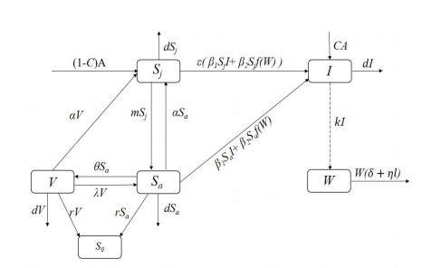
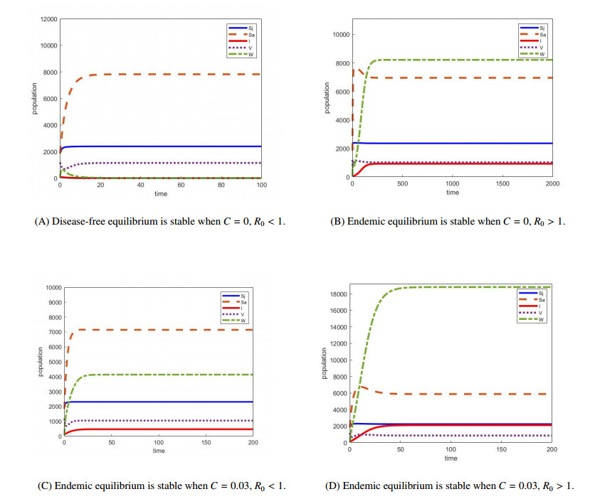
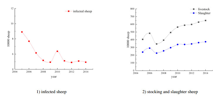
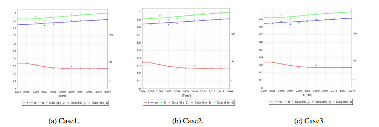
We develop a mathematical model for the transmission of brucellosis in sheep taking into account external inputs, immunity, stage structure and other factors. We find the the basic reproduction number $ R_0 $ in terms of the model parameters, and prove the global stability of the disease-free equilibrium. Then, the existence and global stability of the endemic equilibrium is proven. Finally, sheep data from Yulin, China are employed to fit the model parameters for three different environmental infection exposure conditions. The variability between different models in terms of control measures are analyzed numerically. Results show that the model is sensitive to the control parameters for different environmental infection exposure functions. This means that in practical modeling, the selection of environmental infection exposure functions needs to be properly considered.
- Brucellosis,
- multi-structure,
- environmental infection function,
- control parameter
Citation: Zongmin Yue, Yuanhua Mu, Kekui Yu. Dynamic analysis of sheep Brucellosis model with environmental infection pathways[J]. Mathematical Biosciences and Engineering, 2023, 20(7): 11688-11712. doi: 10.3934/mbe.2023520

Related Papers:

Abstract

We develop a mathematical model for the transmission of brucellosis in sheep taking into account external inputs, immunity, stage structure and other factors. We find the the basic reproduction number $ R_0 $ in terms of the model parameters, and prove the global stability of the disease-free equilibrium. Then, the existence and global stability of the endemic equilibrium is proven. Finally, sheep data from Yulin, China are employed to fit the model parameters for three different environmental infection exposure conditions. The variability between different models in terms of control measures are analyzed numerically. Results show that the model is sensitive to the control parameters for different environmental infection exposure functions. This means that in practical modeling, the selection of environmental infection exposure functions needs to be properly considered.

References

[1]	J. J. Wang, L. Zhang, Current problems and countermeasures in the prevention and control of bovine brucellosis, Chin. Anim. Husb. Vet. Med., 34 (2007), 109. https://doi.org/10.3969/j.issn.1671-7236.2007.03.038 doi: 10.3969/j.issn.1671-7236.2007.03.038
[2]	D. Q. Shang, Research progress of brucellosis, Chin. J. Endemic Dis. Control, 19 (2004), 204–212. https://doi.org/10.3969/j.issn.1001-1889.2004.04.004 doi: 10.3969/j.issn.1001-1889.2004.04.004
[3]	H. L. Ren, S. Y. Lu, Y. Zhou, Z. H. Li, Z. S. Liu, Progress in research and control of Brucellosis, Chin. Anim. Husb. Vet. Med., 36 (2009), 139–143.
[4]	J. P. Gorvel, Brucella: a Mr "Hide" converted into Dr Jekyll, Microbes Infect., 10 (2008), 1010–1013. https://doi.org/10.1016/j.micinf.2008.07.007 doi: 10.1016/j.micinf.2008.07.007
[5]	M. P. Franco, M. Mulder, R. H. Gilman, H. L. Smits, Human brucellosis, Lancet Infect. Dis., 7 (2007), 775–786. https://doi.org/10.1016/S1473-3099(07)70286-4 doi: 10.1016/S1473-3099(07)70286-4
[6]	M. T. Li, G. Q. Sun, W. Y. Zhang, Z. Jin, Model-based evaluation of strategies to control Brucellosis in China, Int. J. Environ. Res. Public Health, 14 (2017), 295. https://doi.org/10.3390/ijerph14030295 doi: 10.3390/ijerph14030295
[7]	X. J. Wang, D. Wang, Y. Y. Shi, C. Q. Xu, A mathematical model analysis of Brucellosis in Inner Mongolia, J. Beijing Univ. Civil Eng. Archit., 32 (2016), 65–69. https://doi.org/10.3969/j.issn.1004-6011.2016.02.013 doi: 10.3969/j.issn.1004-6011.2016.02.013
[8]	C. Li, Z. G. Guo, Z. Y. Zhang, Transmission dynamics of a brucellosis model: Basic reproduction number and global analysis, Chaos, Solitons Fractals, 104 (2017), 161–172. https://doi.org/10.1016/j.chaos.2017.08.013 doi: 10.1016/j.chaos.2017.08.013
[9]	O. Vasilyeva, T. Oraby, F. Lutscher, Aggregation and environmental transmission in chronic wasting disease, Math. Biol. Eng., 12 (2015), 209–231. https://doi.org/10.3934/mbe.2015.12.209 doi: 10.3934/mbe.2015.12.209
[10]	C. J. Shen, M. T. Li, W. Zhang, Y. Yi, Y. Wang, Q. Hou, et al., Modeling transmission dynamics of Streptococcus suis with stage structure and sensitivity analysis, Discrete Dyn. Nat. Soc., 2014 (2014), 1–10. https://doi.org/10.1155/2014/432602 doi: 10.1155/2014/432602
[11]	M. T. Li, G. Q. Sun, Y. F. Wu, J. Zhang, Z. Jin, Transmission dynamics of a multi-group brucellosis model with mixed cross infection in public farm, Appl. Math. Comput., 237 (2014), 582–594. https://doi.org/10.1016/j.amc.2014.03.094 doi: 10.1016/j.amc.2014.03.094
[12]	K. Meng, X. Abdurahman, Study of the brucellosis transmission with multi-stage, Commun. Math. Biol. Neurosci., 2018 (2018). https://doi.org/10.28919/cmbn/3796 doi: 10.28919/cmbn/3796
[13]	X. D. Sun, Q. Hou, Modeling sheep brucellosis transmission with a multi stage model in chanling country of jilin province, Appl. Math. Comput., 51 (2016), 227–244. https://doi.org/10.1007/s12190-015-0901-y doi: 10.1007/s12190-015-0901-y
[14]	P. O. Lolika, S. Mushayabasa, C. P. Bhunu, C. Modnak, J. Wang, Modeling and analyzing the effects of seasonality on brucellosis infection, Chaos, Solitons Fractals, 104 (2017), 338–349. https://doi.org/10.1016/j.chaos.2017.08.027 doi: 10.1016/j.chaos.2017.08.027
[15]	J. Hang, S. G. Ruan, G. Q. Sun, X. Sun, Z. Jin, Analysis of multi-patch dynamical model about cattle brucellosis, J. Shanghai Normal Univ., 43 (2014), 441–455. https://doi.org/10.3969/j.issn.100-5137.2014.05.001 doi: 10.3969/j.issn.100-5137.2014.05.001
[16]	G. Q. Sun, Z. K. Zhang, Global stability for a sheep brucellosis model with immigration, Appl. Math. Comput., 246 (2014), 336–345. https://doi.org/10.1016/j.amc.2014.08.028 doi: 10.1016/j.amc.2014.08.028
[17]	J. B. Muma, N. Toft, J. Oloya, A. Lund, K. Nielsen, K. Samui, et al., Evaluation of three serological tests for brucellosis in naturally infected cattle using latent class analysis, Vet. Microbiol., 125 (2007), 187–192. https://doi.org/10.1016/j.vetmic.2007.05.012 doi: 10.1016/j.vetmic.2007.05.012
[18]	O. Diekmann, J. A. P. Heesterbeek, J. A. J. Metz, On the definition and the computation of the basic reproduction ratio $R_0$ in models for infectious diseases in heterogeneous populations, J. Math. Biol., 28 (1990), 365–382. https://doi.org/10.1007/bf00178324 doi: 10.1007/bf00178324
[19]	O. Diekmann, J. A. P. Heesterbeek, M. G. Roberts, The construction of next-generation matrices for compartmental epidemic models, J. R. Soc. Interface, 7 (2010), 873–885. https://doi.org/10.1098/rsif.2009.0386 doi: 10.1098/rsif.2009.0386
[20]	P. Van den Driessche, J. Watmough, Reproduction numbers and sub-threshold endemic equilibria for compartmental models of disease transmission, Math. Biosci., 180 (2002), 29–48. https://doi.org/10.1016/s0025-5564(02)00108-6 doi: 10.1016/s0025-5564(02)00108-6
[21]	J. P. Lasalle, The Stability of Dynamical Systems, Society for Industrial and Applied Mathematics, 1976. https://doi.org/10.1137/1.9781611970432
[22]	R. P. Sigdel, C. C. McCluskey, Global stability for an it SEI model of infectious disease with immigration, Appl. Math. Comput., 243 (2014), 684–689. https://doi.org/10.1016/j.amc.2014.06.020 doi: 10.1016/j.amc.2014.06.020
[23]	H. Akaike, A new look at the statistical model identification, IEEE Trans. Autom. Control, 19 (1974), 716–723. https://doi.org/10.1007/978-1-4612-1694-0_16 doi: 10.1007/978-1-4612-1694-0_16
[24]	C. M. Hurvich, C. L. Tsai, Regression and time series model selection in small samples, Biometrika, 76 (1989), 297–307. https://doi.org/10.1093/biomet/76.2.297 doi: 10.1093/biomet/76.2.297
[25]	M. De la Sen, R. Nistal, S. Alonso-Quesada, A. Ibeas, Some formal results on positivity, stability, and endemic steady-state attainability based on linear algebraic tools for a class of epidemic models with eventual incommensurate delays, Discrete Dyn. Nat. Soc., 2 (2019), 1–22. https://doi.org/10.1155/2019/8959681 doi: 10.1155/2019/8959681
[26]	S. S. Chen, Y. J. Ran, H. B. Huang, Z. Wang, K. K. Shang, Epidemic dynamics of two-pathogen spreading for pairwise models, Mathematics, 10 (2022), 1906. https://doi.org/10.3390/math10111906 doi: 10.3390/math10111906
[27]	M. De la Sen, S. Alonso-Quesada, A. Ibeas, On the stability of an SEIR epidemic model with distributed time-delay and a general class of feedback vaccination rules, Appl. Math. Comput., 270 (2015), 953–976. https://doi.org/10.1016/j.amc.2015.08.099 doi: 10.1016/j.amc.2015.08.099
[28]	R. Xu, Global dynamics of a delayed epidemic model with latency and relapse, Nonlinear Anal.-Model. Control, 18 (2013), 250–263. https://doi.org/10.15388/NA.18.2.14026 doi: 10.15388/NA.18.2.14026

Reader Comments

Your name:*

Email:*
© 2023 the Author(s), licensee AIMS Press. This is an open access article distributed under the terms of the Creative Commons Attribution License (http://creativecommons.org/licenses/by/4.0)