We consider the following chemotaxis-growth system with an acceleration assumption,
$ \begin{align*} \begin{cases} u_t= \Delta u -\nabla \cdot\left(u \mathbf{w} \right)+\gamma\left({u-u^\alpha}\right), & x\in\Omega,\ t>0,\\ v_t=\Delta v- v+u, & x\in\Omega,\ t>0,\\ \mathbf{w}_t= \Delta \mathbf{w} - \mathbf{w} +\chi\nabla v, & x\in\Omega,\ t>0, \end{cases} \end{align*} $
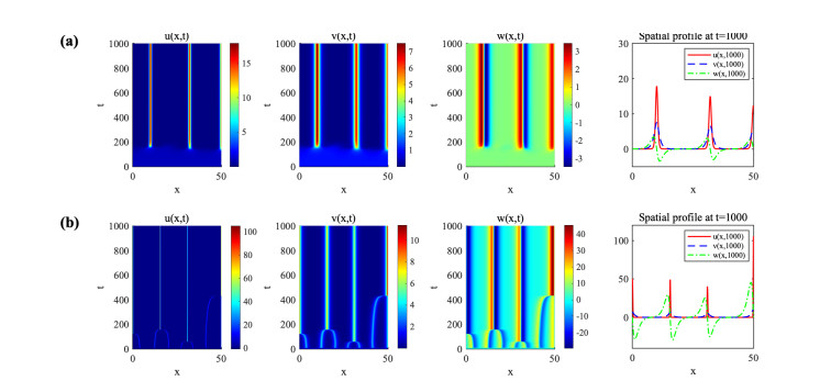
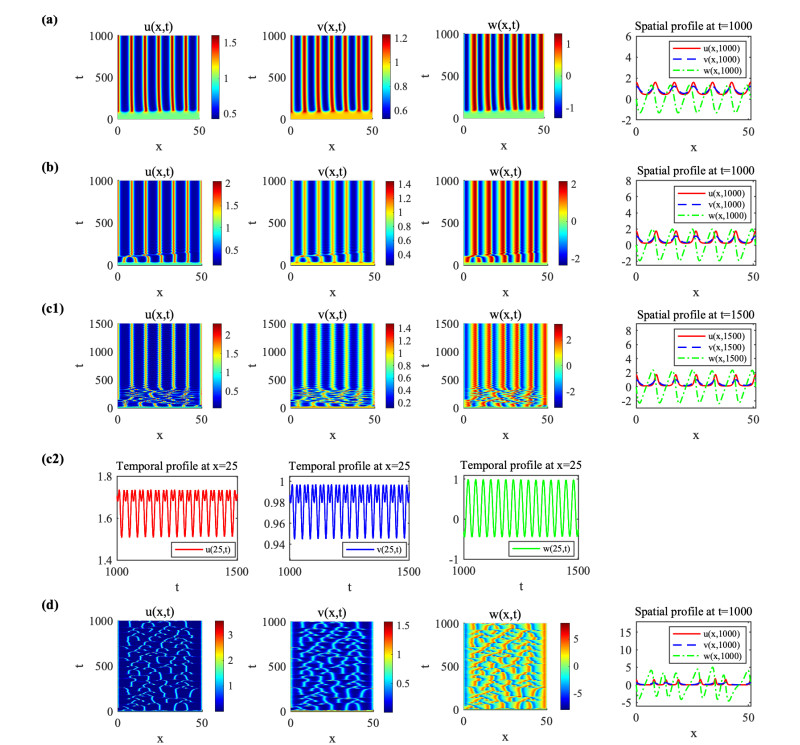
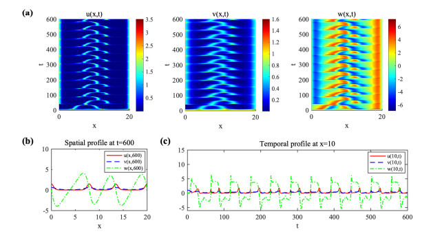
under the homogeneous Neumann boundary condition for $ u, v $ and the homogeneous Dirichlet boundary condition for $ \mathbf{w} $ in a smooth bounded domain $ \Omega\subset \mathbb{R}^{n} $ ($ n\geq1 $) with given parameters $ \chi > 0 $, $ \gamma\geq0 $ and $ \alpha > 1 $. It is proved that for reasonable initial data with either $ n\leq3 $, $ \gamma\geq0 $, $ \alpha > 1 $ or $ n\geq4, \ \gamma > 0, \ \alpha > \frac12+\frac n4 $, the system admits global bounded solutions, which significantly differs from the classical chemotaxis model that may have blow-up solutions in two and three dimensions. For given $ \gamma $ and $ \alpha $, the obtained global bounded solutions are shown to convergence exponentially to the spatially homogeneous steady state $ (m, m, \bf 0 $) in the large time limit for appropriately small $ \chi $, where $ m = \frac1{|\Omega|} \int_\Omega u_0(x) $ if $ \gamma = 0 $ and $ m = 1 $ if $ \gamma > 0 $. Outside the stable parameter regime, we conduct linear analysis to specify possible patterning regimes. In weakly nonlinear parameter regimes, with a standard perturbation expansion approach, we show that the above asymmetric model can generate pitchfork bifurcations which occur generically in symmetric systems. Moreover, our numerical simulations demonstrate that the model can generate rich aggregation patterns, including stationary, single merging aggregation, merging and emerging chaotic, and spatially inhomogeneous time-periodic. Some open questions for further research are discussed.
Citation: Chunlai Mu, Weirun Tao. Stabilization and pattern formation in chemotaxis models with acceleration and logistic source[J]. Mathematical Biosciences and Engineering, 2023, 20(2): 2011-2038. doi: 10.3934/mbe.2023093
We consider the following chemotaxis-growth system with an acceleration assumption,
$ \begin{align*} \begin{cases} u_t= \Delta u -\nabla \cdot\left(u \mathbf{w} \right)+\gamma\left({u-u^\alpha}\right), & x\in\Omega,\ t>0,\\ v_t=\Delta v- v+u, & x\in\Omega,\ t>0,\\ \mathbf{w}_t= \Delta \mathbf{w} - \mathbf{w} +\chi\nabla v, & x\in\Omega,\ t>0, \end{cases} \end{align*} $
under the homogeneous Neumann boundary condition for $ u, v $ and the homogeneous Dirichlet boundary condition for $ \mathbf{w} $ in a smooth bounded domain $ \Omega\subset \mathbb{R}^{n} $ ($ n\geq1 $) with given parameters $ \chi > 0 $, $ \gamma\geq0 $ and $ \alpha > 1 $. It is proved that for reasonable initial data with either $ n\leq3 $, $ \gamma\geq0 $, $ \alpha > 1 $ or $ n\geq4, \ \gamma > 0, \ \alpha > \frac12+\frac n4 $, the system admits global bounded solutions, which significantly differs from the classical chemotaxis model that may have blow-up solutions in two and three dimensions. For given $ \gamma $ and $ \alpha $, the obtained global bounded solutions are shown to convergence exponentially to the spatially homogeneous steady state $ (m, m, \bf 0 $) in the large time limit for appropriately small $ \chi $, where $ m = \frac1{|\Omega|} \int_\Omega u_0(x) $ if $ \gamma = 0 $ and $ m = 1 $ if $ \gamma > 0 $. Outside the stable parameter regime, we conduct linear analysis to specify possible patterning regimes. In weakly nonlinear parameter regimes, with a standard perturbation expansion approach, we show that the above asymmetric model can generate pitchfork bifurcations which occur generically in symmetric systems. Moreover, our numerical simulations demonstrate that the model can generate rich aggregation patterns, including stationary, single merging aggregation, merging and emerging chaotic, and spatially inhomogeneous time-periodic. Some open questions for further research are discussed.

| [1] |
E. F. Keller, L. A. Segel, Initiation of slime mold aggregation is viewed as an instability, J. Theor. Biol., 26 (1970), 399–415. https://doi.org/10.1016/0022-5193(70)90092-5 doi: 10.1016/0022-5193(70)90092-5

|
| [2] |
N. Bellomo, A. Bellouquid, Y. Tao, M. Winkler, Toward a mathematical theory of Keller-Segel models of pattern formation in biological tissues, Math. Models Methods Appl. Sci., 25 (2015), 1663–1763. https://doi.org/10.1142/S021820251550044X doi: 10.1142/S021820251550044X
|
| [3] |
N. Bellomo, N. Outada, J. Soler, Y. Tao, M. Winkler, Chemotaxis and cross-diffusion models in complex environments: models and analytic problems toward a multiscale vision, Math. Models Methods Appl. Sci., 32 (2022), 713–792. https://doi.org/10.1142/S0218202522500166 doi: 10.1142/S0218202522500166
|
| [4] |
T. Hillen, K. Painter, A user's guide to PDE models for chemotaxis, J. Math. Biol., 58 (2009), 183–217. http://dx.doi.org/10.1007/s00285-008-0201-3 doi: 10.1007/s00285-008-0201-3
|
| [5] | D. Horstmann, From 1970 until present: the Keller-Segel model in chemotaxis and its consequences. II, Jahresber. Deutsch. Math.-Verein., 106 (2004), 51–69. |
| [6] |
P. Kareiva, G. Odell, Swarms of predators exhibit "preytaxis" if individual predators use area-restricted search, Amer. Natur., 130 (1987), 233–270. https://doi.org/10.1086/284707 doi: 10.1086/284707
|
| [7] |
G. R. Flierl, D. Grünbaum, S. A. Levins, D. B. Olson, From individuals to aggregations: the interplay between behavior and physics, J. Theor. Biol., 196 (1999), 397–454. https://doi.org/10.1006/jtbi.1998.0842 doi: 10.1006/jtbi.1998.0842
|
| [8] |
A. Okubo, H. C. Chiang, C. C. Ebbesmeyer, Acceleration field of individual midges, anarete pritchardi (diptera: Cecidomyiidae), within a swarm, Can. Entomol., 109 (1977), 149–156. https://doi.org/10.4039/Ent109149-1 doi: 10.4039/Ent109149-1
|
| [9] | J. K. Parrish, P. Turchin, Individual decisions, traffic rules, and emergent pattern in schooling fish, Animal groups in three dimensions, Cambridge University Press, Cambridge, 126–142. |
| [10] |
P. Kareiva, Experimental and mathematical analyses of herbivore movement: quantifying the influence of plant spacing and quality on foraging discrimination, Ecol. Monogr., 52 (1982), 261–282. https://doi.org/10.2307/2937331 doi: 10.2307/2937331
|
| [11] |
R. Arditi, Y. Tyutyunov, A. Morgulis, V. Govorukhin, I. Senina, Directed movement of predators and the emergence of density-dependence in predator-prey models, Theor. Popul. Biol., 59 (2001), 207–221. https://doi.org/10.1006/tpbi.2001.1513 doi: 10.1006/tpbi.2001.1513
|
| [12] |
N. Sapoukhina, Y. Tyutyunov, R. Arditi, The role of prey taxis in biological control: a spatial theoretical model, Amer. Nat., 162 (2003), 61–76. https://doi.org/10.1086/375297 doi: 10.1086/375297
|
| [13] |
H.-Y. Jin, Z.-A. Wang, Global dynamics and Spatio-temporal patterns of predator-prey systems with density-dependent motion, European J. Appl. Math., 32 (2021), 652–682. https://doi.org/10.1017/s0956792520000248 doi: 10.1017/s0956792520000248
|
| [14] |
F. Yi, J. Wei, J. Shi, Bifurcation and spatiotemporal patterns in a homogeneous diffusive predator-prey system, J. Differ. Equ., 246 (2009), 1944–1977. https://doi.org/10.1016/j.jde.2008.10.024 doi: 10.1016/j.jde.2008.10.024
|
| [15] | W. Tao, Z.-A. Wang, On a new type of chemotaxis model with acceleration, Commun. Math. Anal. Appl., 1 (2022), 319–344. |
| [16] |
M. A. Herrero, J. J. L. Velázquez, Chemotactic collapse for the Keller-Segel model, J. Math. Biol., 35 (1996), 177–194. https://doi.org/10.1007/s002850050049 doi: 10.1007/s002850050049
|
| [17] |
D. Horstmann, G. Wang, Blow-up in a chemotaxis model without symmetry assumptions, European J. Appl. Math., 12 (2001), 159–177. https://doi.org/10.1017/S0956792501004363 doi: 10.1017/S0956792501004363
|
| [18] | T. Nagai, Blow-up of radially symmetric solutions to a chemotaxis system, Adv. Math. Sci. Appl., 5 (1995), 581–601. |
| [19] |
T. Nagai, Blowup of nonradial solutions to parabolic-elliptic systems modeling chemotaxis in two-dimensional domains, J. Inequal. Appl., 6 (2001), 37–55. https://doi.org/10.1155/S1025583401000042 doi: 10.1155/S1025583401000042
|
| [20] | T. Nagai, T. Senba, K. Yoshida, Application of the Trudinger-Moser inequality to a parabolic system of chemotaxis, Funkcial. Ekvac., 40 (1997), 411–433. |
| [21] |
M. Winkler, Finite-time blow-up in the higher-dimensional parabolic-parabolic Keller-Segel system, J. Math. Pures Appl., 100 (2013), 748–767. https://doi.org/10.1016/j.matpur.2013.01.020 doi: 10.1016/j.matpur.2013.01.020
|
| [22] |
A. Blanchet, J. A. Carrillo, P. Laurençot, Critical mass for a Patlak-Keller-Segel model with degenerate diffusion in higher dimensions, Calc. Var. Part. Differ. Equ., 35 (2009), 133–168. https://doi.org/10.1007/s00526-008-0200-7 doi: 10.1007/s00526-008-0200-7
|
| [23] | A. Blanchet, J. Dolbeault, B. Perthame, Two-dimensional Keller-Segel model: optimal critical mass and qualitative properties of the solutions, Electron. J. Differ. Equ., 2006 (2006), 1–33. https://ejde.math.txstate.edu |
| [24] | V. Calvez, B. Perthame, M. Sharifi tabar, Modified Keller-Segel system and critical mass for the log interaction kernel, in Stochastic analysis and partial differential equations, vol. 429 of Contemp. Math., Amer. Math. Soc., Providence, RI, 2007, 45–62. https://doi.org/10.1090/conm/429/08229 |
| [25] |
J. Fuhrmann, J. Lankeit, M. Winkler, A double critical mass phenomenon in a no-flux-Dirichlet Keller-Segel system, J. Math. Pures Appl., 162 (2022), 124–151. https://doi.org/10.1016/j.matpur.2022.04.004 doi: 10.1016/j.matpur.2022.04.004
|
| [26] | K. Fujie, J. Jiang, Comparison methods for a Keller-Segel-type model of pattern formations with density-suppressed motilities, Calc. Var. Part. Differ. Equ., 60 (2021), Paper No. 92, 37, https://doi.org/10.1007/s00526-021-01943-5 |
| [27] |
H.-Y. Jin, Z.-A. Wang, Boundedness, blowup and critical mass phenomenon in competing for chemotaxis, J. Differ. Equ., 260 (2016), 162–196. https://doi.org/10.1016/j.jde.2015.08.040 doi: 10.1016/j.jde.2015.08.040
|
| [28] |
H.-Y. Jin, Z.-A. Wang, Critical mass on the Keller-Segel system with signal-dependent motility, Proc. Amer. Math. Soc., 148 (2020), 4855–4873. https://doi.org/10.1090/proc/15124 doi: 10.1090/proc/15124
|
| [29] |
Y. Tao, M. Winkler, Critical mass for infinite-time aggregation in a chemotaxis model with indirect signal production, J. Eur. Math. Soc., 19 (2017), 3641–3678. https://doi.org/10.4171/JEMS/749 doi: 10.4171/JEMS/749
|
| [30] | J. I. Tello, M. Winkler, Reduction of critical mass in a chemotaxis system by external application of a chemoattractant, Ann. Sc. Norm. Super. Pisa Cl. Sci., 12 (2013), 833–862. |
| [31] |
M. Winkler, How unstable is spatial homogeneity in Keller-Segel systems? A new critical mass phenomenon in two- and higher-dimensional parabolic-elliptic cases, Math. Ann., 373 (2019), 1237–1282. https://doi.org/10.1007/s00208-018-1722-8 doi: 10.1007/s00208-018-1722-8
|
| [32] |
M. Winkler, Can fluid interaction influence the critical mass for taxis-driven blow-up in bounded planar domains?, Acta Appl. Math., 169 (2020), 577–591. https://doi.org/10.1007/s10440-020-00312-2 doi: 10.1007/s10440-020-00312-2
|
| [33] |
M. Winkler, A family of mass-critical Keller-Segel systems, Proc. Lond. Math. Soc., 124 (2022), 133–181. https://doi.org/10.1112/plms.12425 doi: 10.1112/plms.12425
|
| [34] |
K. Osaki, T. Tsujikawa, A. Yagi, M. Mimura, Exponential attractor for a chemotaxis-growth system of equations, Nonlinear Anal., 51 (2002), 119–144. https://doi.org/10.1016/S0362-546X(01)00815-X doi: 10.1016/S0362-546X(01)00815-X
|
| [35] |
R. B. Salako, W. Shen, Global existence and asymptotic behavior of classical solutions to a parabolic–elliptic chemotaxis system with logistic source on rn, J. Differ. Equ., 262 (2017), 5635–5690. https://doi.org/10.1016/j.jde.2017.02.011 doi: 10.1016/j.jde.2017.02.011
|
| [36] |
J. I. Tello, M. Winkler, A chemotaxis system with logistic source, Comm. Part. Differ. Equ., 32 (2007), 849–877. https://doi.org/10.1080/03605300701319003 doi: 10.1080/03605300701319003
|
| [37] |
M. Winkler, Boundedness in the higher-dimensional parabolic-parabolic chemotaxis system with logistic source, Comm. Part. Differ. Equ., 35 (2010), 1516–1537. https://doi.org/10.1080/03605300903473426 doi: 10.1080/03605300903473426
|
| [38] |
T. Xiang, Boundedness and global existence in the higher-dimensional parabolic-parabolic chemotaxis system with/without growth source, J. Differ. Equ., 258 (2015), 4275–4323. https://doi.org/10.1016/j.jde.2015.01.032 doi: 10.1016/j.jde.2015.01.032
|
| [39] | M. Winkler, Finite-time blow-up in low-dimensional Keller-Segel systems with logistic-type superlinear degradation, Z. Angew. Math. Phys., 69 (2018), Paper No. 69, 40. https://doi.org/10.1007/s00033-018-0935-8 |
| [40] |
K. Fujie, T. Senba, Application of an Adams type inequality to a two-chemical substances chemotaxis system, J. Differ. Equ., 263 (2017), 88–148. https://doi.org/10.1016/j.jde.2017.02.031 doi: 10.1016/j.jde.2017.02.031
|
| [41] |
W. Zhang, P. Niu, S. Liu, Large time behavior in a chemotaxis model with logistic growth and indirect signal production, Nonlinear Anal. Real World Appl., 50 (2019), 484–497. https://doi.org/10.1016/j.nonrwa.2019.05.002 doi: 10.1016/j.nonrwa.2019.05.002
|
| [42] |
H. Li, Y. Tao, Boundedness in a chemotaxis system with indirect signal production and generalized logistic source, Appl. Math. Lett., 77 (2018), 108–113. https://doi.org/10.1016/j.aml.2017.10.006 doi: 10.1016/j.aml.2017.10.006
|
| [43] |
K. J. Painter, T. Hillen, Spatio-temporal chaos in a chemotaxis model, Physica D, 240 (2011), 363–375, https://doi.org/10.1016/j.physd.2010.09.011. doi: 10.1016/j.physd.2010.09.011
|
| [44] | M. Cross, H. Greenside, Pattern formation and dynamics in nonequilibrium systems, Cambridge University Press, 2009. |
| [45] |
T. Hillen, J. Zielinski, K. J. Painter, Merging-emerging systems can describe spatio-temporal patterning in a chemotaxis model, Discrete Contin. Dyn. Syst. Ser. B, 18 (2013), 2513–2536. https://doi.org/10.3934/dcdsb.2013.18.2513 doi: 10.3934/dcdsb.2013.18.2513
|
| [46] |
D. Horstmann, M. Winkler, Boundedness vs. blow-up in a chemotaxis system, J. Differ. Equ., 215 (2005), 52–107. https://doi.org/10.1016/j.jde.2004.10.022 doi: 10.1016/j.jde.2004.10.022
|
| [47] |
H.-Y. Jin and Z.-A. Wang, Global stability of prey-taxis systems, J. Differ. Equ., 262 (2017), 1257–1290. https://doi.org/10.1016/j.jde.2016.10.010 doi: 10.1016/j.jde.2016.10.010
|
| [48] |
H.-Y. Jin, Z.-A. Wang, Global stabilization of the full attraction-repulsion Keller-Segel system, Discrete Contin. Dyn. Syst., 40 (2020), 3509–3527. https://doi.org/10.3934/dcds.2020027 doi: 10.3934/dcds.2020027
|
| [49] |
R. Kowalczyk, Z. Szymańska, On the global existence of solutions to an aggregation model, J. Math. Anal. Appl., 343 (2008), 379–398. https://doi.org/10.1016/j.jmaa.2008.01.005 doi: 10.1016/j.jmaa.2008.01.005
|
| [50] |
G. Li, Y. Yao, Two-species competition model with chemotaxis: well-posedness, stability and dynamics, Nonlinearity, 35 (2022), 1329–1359. https://doi.org/10.1088/1361-6544/ac4a8d doi: 10.1088/1361-6544/ac4a8d
|
| [51] | G. M. Lieberman, Second order parabolic differential equations, World Scientific Publishing Co., Inc., River Edge, NJ, 1996. https: //doi.org/10.1142/3302 |
| [52] |
P. Liu, J. Shi, Z.-A. Wang, Pattern formation of the attraction-repulsion Keller-Segel system, Discrete Contin. Dyn. Syst. Ser. B, 18 (2013), 2597–2625. https://doi.org/10.3934/dcdsb.2013.18.2597 doi: 10.3934/dcdsb.2013.18.2597
|
| [53] |
M. Ma, C. Ou, Z.-A. Wang, Stationary solutions of a volume-filling chemotaxis model with logistic growth and their stability, SIAM J. Appl. Math., 72 (2012), 740–766. https://doi.org/10.1137/110843964 doi: 10.1137/110843964
|
| [54] |
M. Ma, Z.-A. Wang, Global bifurcation and stability of steady states for a reaction-diffusion-chemotaxis model with volume-filling effect, Nonlinearity, 28 (2015), 2639–2660. https://doi.org/10.1088/0951-7715/28/8/2639 doi: 10.1088/0951-7715/28/8/2639
|
| [55] | C. Mu, W. Tao, Z.-A. Wang, Global dynamics and spatiotemporal heterogeneity of accelerated preytaxis models, preprint. |
| [56] | J. D. Murray, Mathematical Biology I: An introduction, vol. 17 of Interdisciplinary Applied Mathematics, 3rd edition, Springer-Verlag, New York, 2002. |
| [57] | K. J. Painter, T. Hillen, Volume-filling and quorum-sensing in models for chemosensitive movement, Can. Appl. Math. Q., 10 (2002), 501–543. |
| [58] | P. Quittner, P. Souplet, Superlinear parabolic problems. Blow-up, global existence and steady states, Birkhäuser, Basel, 2019. |
| [59] |
Y. Tao, M. Winkler, Boundedness and decay enforced by quadratic degradation in a three-dimensional chemotaxis–fluid system, Z. Angew. Math. Phys., 66 (2015), 2555–2573. https://doi.org/10.1007/s00033-015-0541-y doi: 10.1007/s00033-015-0541-y
|
| [60] |
J. Wang, M. Wang, The dynamics of a predator-prey model with diffusion and indirect prey-taxis, J. Dyn. Differ. Equ., 32 (2020), 1291–1310. https://doi.org/10.1007/s10884-019-09778-7 doi: 10.1007/s10884-019-09778-7
|
| [61] |
M. Wang, Note on the Lyapunov functional method, Appl. Math. Lett., 75 (2018), 102–107. https://doi.org/10.1016/j.aml.2017.07.003 doi: 10.1016/j.aml.2017.07.003
|
| [62] |
Z. Wang, T. Hillen, Classical solutions and pattern formation for a volume filling chemotaxis model, Chaos, 17 (2007), 037108, 13. https://doi.org/10.1063/1.2766864 doi: 10.1063/1.2766864
|
| [63] |
M. Winkler, Aggregation vs. global diffusive behavior in the higher-dimensional Keller-Segel model, J. Differ. Equ., 248 (2010), 2889–2905. http://dx.doi.org/10.1016/j.jde.2010.02.008 doi: 10.1016/j.jde.2010.02.008
|
Figures(3)

Chunlai Mu, Weirun Tao. Stabilization and pattern formation in chemotaxis models with acceleration and logistic source[J]. Mathematical Biosciences and Engineering, 2023, 20(2): 2011-2038. doi: 10.3934/mbe.2023093


 DownLoad: