Modelling and stability analysis of ASFV with swill and the virus in the environment

Haitao Song; Lirong Guo; Zhen Jin; Shengqiang Liu; Haitao Song; Lirong Guo; Zhen Jin; Shengqiang Liu

doi:10.3934/mbe.2022608

Mathematical Biosciences and Engineering

2022, Volume 19, Issue 12: 13028-13049. doi: 10.3934/mbe.2022608

Previous Article Next Article

Research article Special Issues

Modelling and stability analysis of ASFV with swill and the virus in the environment

1.
Complex Systems Research Center, Shanxi University, Taiyuan 030006, China
2.
Shanxi Key Laboratory of Mathematical Techniques and Big Data Analysis, on disease Control and Prevention, Shanxi University, Taiyuan 030006, China
3.
School of Mathematical Sciences, Shanxi University, Taiyuan 030006, China
4.
School of Mathematical Sciences, Tiangong University, Tianjin 300387, China

Academic Editor: Sanling Yuan

Received: 17 June 2022 Revised: 22 August 2022 Accepted: 29 August 2022 Published: 05 September 2022

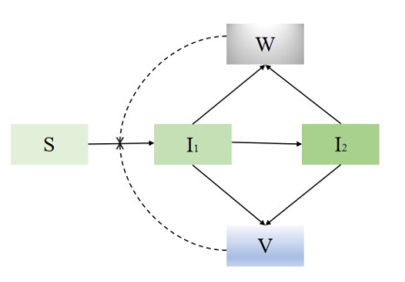
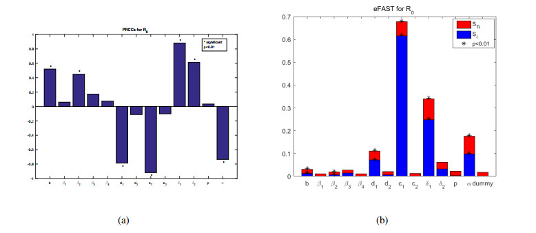
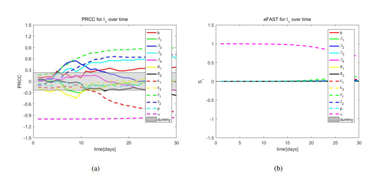
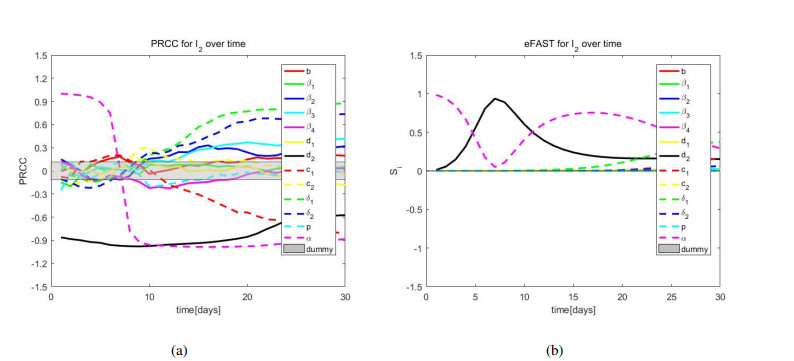
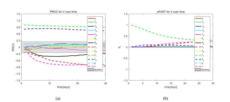
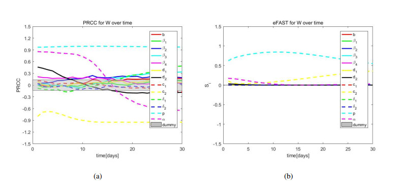
African swine fever (ASF) is an acute, hemorrhagic and severe infectious disease caused by the African swine fever virus (ASFV), and leads to a serious threat to the pig industry in China. Yet the impact of the virus in the environment and contaminated swill on the ASFV transmission is unclear in China. Then we build the ASFV transmission model with the virus in the environment and swill. We compute the basic reproduction number, and prove that the disease-free equilibrium is globally asymptotically stable when $ R_0 < 1 $ and the unique endemic equilibrium is globally asymptotically stable when $ R_0 > 1 $. Using the public information, parameter values are evaluated. PRCCs and eFAST sensitivity analysis reveal that the release rate of ASFV from asymptomatic and symptomatic infectious pigs and the proportion of pig products from infectious pigs to swill have a significant impact on the ASFV transmission. Our findings suggest that the virus in the environment and contaminated swill contribute to the ASFV transmission. Our results may help animal health to prevent and control the ASFV transmission.
- African swine fever,
- mathematical model,
- swill,
- sensitivity analysis,
- global stability
Citation: Haitao Song, Lirong Guo, Zhen Jin, Shengqiang Liu. Modelling and stability analysis of ASFV with swill and the virus in the environment[J]. Mathematical Biosciences and Engineering, 2022, 19(12): 13028-13049. doi: 10.3934/mbe.2022608

Related Papers:

Abstract

African swine fever (ASF) is an acute, hemorrhagic and severe infectious disease caused by the African swine fever virus (ASFV), and leads to a serious threat to the pig industry in China. Yet the impact of the virus in the environment and contaminated swill on the ASFV transmission is unclear in China. Then we build the ASFV transmission model with the virus in the environment and swill. We compute the basic reproduction number, and prove that the disease-free equilibrium is globally asymptotically stable when $ R_0 < 1 $ and the unique endemic equilibrium is globally asymptotically stable when $ R_0 > 1 $. Using the public information, parameter values are evaluated. PRCCs and eFAST sensitivity analysis reveal that the release rate of ASFV from asymptomatic and symptomatic infectious pigs and the proportion of pig products from infectious pigs to swill have a significant impact on the ASFV transmission. Our findings suggest that the virus in the environment and contaminated swill contribute to the ASFV transmission. Our results may help animal health to prevent and control the ASFV transmission.

References

[1]	C. Alonso, M. Borca, L. Dixon, Y Revilla, F. ROdriguez, J. M. Escribano, ICTV virus taxonomy profile: Asfarviridae, J. Gen. Virol., 99 (2018), 613–614. https://doi.org/10.1099/jgv.0.001049 doi: 10.1099/jgv.0.001049
[2]	C. M. Fauquet, M. A. Mayo, J. Maniloff, U. Desselberger, L. A. Ball, Virus taxonomy: VIIIth report of the International Committee on Taxonomy of Viruses, Academic Press, 2005.
[3]	S. Costard, B. Wieland, W. De Glanville, F. Jori, R. Rowlands, W. Vosloo, et al., African swine fever: how can global spread be prevented?, Phil. Trans. R. Soc. B, 364 (2009), 2683–2696. https://doi.org/10.1098/rstb.2009.0098 doi: 10.1098/rstb.2009.0098
[4]	C. Guinat, A. Gogin, S. Blome, G. Keil, R. Pollin, D. U. Pfeiffer, et al., Transmission routes of African swine fever virus to domestic pigs: current knowledge and future research directions, Vet. Rec., 178 (2016), 262–267. https://doi.org/10.1136/vr.103593 doi: 10.1136/vr.103593
[5]	H. Nishiura, Early efforts in modeling the incubation period of infectious diseases with an acute course of illness, Emerg. Themes Epidemiology, 4 (2007), 1–12. https://doi.org/10.1186/1742-7622-4-2 doi: 10.1186/1742-7622-4-2
[6]	I. Galindo, C. Alonso, African swine fever virus: a review, Viruses, 9 (2017), 103. https://doi.org/10.3390/v9050103 doi: 10.3390/v9050103
[7]	C. J. Quembo, F. Jori, W. Vosloo, L. Health, Genetic characterization of African swine fever virus isolates from soft ticks at the wildlife/domestic interface in Mozambique and identification of a novel genotype, Transbound. Emerg. Dis., 65 (2018), 420–431. https://doi.org/10.1111/tbed.12700 doi: 10.1111/tbed.12700
[8]	E. R. Tulman, G. A. Delhon, B. K. Ku, D. L. Rock, African Swine Fever Virus. In: Van Etten, J.L. (eds) Lesser Known Large dsDNA Viruses. Current Topics in Microbiology and Immunology, Springer, Berlin, Heidelberg, 2009. https://doi.org/10.1007/978-3-540-68618-7_2
[9]	X. Shen, Z. Pu, Y. Li, S. Yu, F. Guo, T. Luo, et al., Phylogeographic patterns of the African swine fever virus, J. Infect., 79 (2019), 174–187. https://doi.org/10.1016/j.jinf.2019.05.004 doi: 10.1016/j.jinf.2019.05.004
[10]	T. Wang, Y. Sun, H. J. Qiu, African swine fever: an unprecedented disaster and challenge to China, Infec. Dis. Poverty, 7 (2018), 66–70. https://doi.org/10.1186/s40249-018-0495-3 doi: 10.1186/s40249-018-0495-3
[11]	J. Bao, Q. Wang, P. Lin, C. Liu, L. Li, X. Wu, et al., Genome comparison of African swine fever virus China/2018/AnhuiXCGQ strain and related European p72 Genotype II strains, Transbound. Emerg. Dis., 66 (2019), 1167–1176. https://doi.org/10.1111/tbed.13124 doi: 10.1111/tbed.13124
[12]	X. Zhou, N. Li, Y. Luo, Y. E. Liu, F. Miao, T. Chen, et al., Emergence of African swine fever in China, 2018, Transbound. Emerg. Dis., 65 (2018), 1482–1484. https://doi.org/10.1111/tbed.12989 doi: 10.1111/tbed.12989
[13]	S. Ge, J. Li, X. Fan, F. Liu, L. Li, Q. Wang, et al., Molecular characterization of African swine fever virus, China, 2018, Emerg. Infect. Dis., 24 (2018), 2131–2133. https://doi.org/10.3201/eid2411.181274 doi: 10.3201/eid2411.181274
[14]	Q. Wang, W. Ren, J. Bao, S. Ge, J. Li, L. Li, et al., The first outbreak of African swine fever was confirmed in China, China Animal Health Inspection, 35 (2018), 1–4. https://doi.org/10.3969/j.issn.1005-944X.2018.09.001 doi: 10.3969/j.issn.1005-944X.2018.09.001
[15]	Y. Wang, L. Gao, Y. Li, Q. Xu, H. Yang, C. Shen, et al., African swine fever in China: Emergence and control, J. Biosaf. Biosecur., 1 (2019), 7–8. https://doi.org/10.1016/j.jobb.2019.01.006 doi: 10.1016/j.jobb.2019.01.006
[16]	H. Song, W. Jiang, S. Liu, Global dynamics of two heterogeneous SIR models with nonlinear incidence and delays, Int. J. Biomath., 9 (2016), 1650046. https://doi.org/10.1142/S1793524516500467 doi: 10.1142/S1793524516500467
[17]	H. Song, S. Liu, W. Jiang, Global dynamics of a multistage SIR model with distributed delays and nonlinear incidence rate, Math. Methods Appl. Sci., 40 (2017), 2153–2164. https://doi.org/10.1002/mma.4130 doi: 10.1002/mma.4130
[18]	H. Song, F. Li, Z. Jia, Z. Jin, S. Liu, Using traveller-derived cases in Henan Province to quantify the spread of COVID-19 in Wuhan, China, Nonlinear Dyn., 101 (2020), 1821–1831. https://doi.org/10.1007/s11071-020-05859-1 doi: 10.1007/s11071-020-05859-1
[19]	H. Song, Z. Jia, Z. Jin, S. Liu, Estimation of COVID-19 outbreak size in Harbin, China, Nonlinear Dyn., 106 (2021), 1229–1237. https://doi.org/10.1007/s11071-021-06406-2 doi: 10.1007/s11071-021-06406-2
[20]	H. Song, G. Fan, S. Zhao, H. Li, Q. Huang, D. He, Forecast of the COVID-19 trend in India: a simple modelling approach, Math. Biosci. Eng., 18 (2021), 9775–9786. https://doi.org/10.3934/mbe.2021479 doi: 10.3934/mbe.2021479
[21]	H. Song, G. Fan, Y. Liu, X. Wang, D. He, The Second Wave of COVID-19 in South and Southeast Asia and the Effects of Vaccination, Front. Med., 8 (2021), 773110. https://doi.org/10.3389/fmed.2021.773110 doi: 10.3389/fmed.2021.773110
[22]	H. Song, F. Liu, F. Li, C. Cao, H. Wang, Z. Jia, et al., Modeling the second outbreak of COVID-19 with isolation and contact tracing, Discrete Cont. Dyn.-B, 27 (2022), 5757–5777. https://doi.org/10.3934/dcdsb.2021294 doi: 10.3934/dcdsb.2021294
[23]	H. Song, Z. Jin, C. Shan, L. Chang, The spatial and temporal effects of Fog-Haze pollution on the influenza transmission, Int. J. Biomath., (2022), 2250096. https://doi.org/10.1142/S1793524522500966
[24]	F. I. Korennoy, V. M. Gulenkin, A. E. Gogin, T. Vergne, A. K. Karaulov, Estimating the basic reproductive number for African swine fever using the Ukrainian historical epidemic of 1977, Transbound. Emerg. Dis., 64 (2017), 1858–1866. https://doi.org/10.1111/tbed.12583 doi: 10.1111/tbed.12583
[25]	C. Guinat, A. L. Reis, C. L. Netherton, L. Goatley, D. U. Pfeiffer, L.Dixon, Dynamics of African swine fever virus shedding and excretion in domestic pigs infected by intramuscular inoculation and contact transmission, Vet. Res., 45 (2014), 1–9. https://doi.org/10.1186/s13567-014-0093-8 doi: 10.1186/s13567-014-0093-8
[26]	M. B. Barongo, R. P. Bishop, E. M. Fevre, D. L. Knobel, A. Ssematimba, A mathematical model that simulates control options for African swine fever virus (ASFV), PLoS One, 11 (2016), e0158658. https://doi.org/10.1371/journal.pone.0158658 doi: 10.1371/journal.pone.0158658
[27]	X. O'Neill, A. White, F. Ruiz-Fons, C. Gortazar, Modelling the transmission and persistence of African swine fever in wild boar in contrasting European scenarios, Sci. Rep., 10 (2020), 1–10. https://doi.org/10.1038/s41598-020-62736-y doi: 10.1038/s41598-020-62736-y
[28]	J. Li, Z. Jin, Y. Wang, X. Sun, Q. Xu, J. Kang, et al., Data-driven dynamical modelling of the transmission of African swine fever in a few places in China, Transbound. Emerg. Dis., 69 (2021), e646–e658. https://doi.org/10.1111/tbed.14345. doi: 10.1111/tbed.14345
[29]	J. M. Sanchez-Vizcaino, L. Mur, J. C. Gomez-Villamandos, L. Carrasco, An update on the epidemiology and pathology of African swine fever, J. Comp. Pathol., 152 (2015), 9–21. https://doi.org/10.1016/j.jcpa.2014.09.003 doi: 10.1016/j.jcpa.2014.09.003
[30]	M. Arias, J. M. Sanchez-Vizcaino, A. Morilla, K. J. Yoon, J. J. Zimmerman, African swine fever, Trends in emerging viral infections of swine, (2002), 119–124.
[31]	H. K. Khalil, Nonlinear Systems, New York: Macmillan Co., 1992.
[32]	P. van den Driessche, J. Watmough, Reproduction numbers and sub-threshold endemic equilibria for compartmental models of disease transmission, Math. Biosci., 180 (2002), 29–48. https://doi.org/10.1016/S0025-5564(02)00108-6 doi: 10.1016/S0025-5564(02)00108-6
[33]	Lasalle J. The Stability of Dynamical Systems, SIAM, Philadelphia, 1976.
[34]	The China Animal Health Endemic Center, https://www.cahec.cn/.
[35]	X. Zhang, X. Rong, J. Li, M. Fan, Y. Wang, X. Sun, et al., Modeling the outbreak and control of African swine fever virus in large-scale pig farms, J. Theor. Biol., 526 (2021), 110798. https://doi.org/10.1016/j.jtbi.2021.110798 doi: 10.1016/j.jtbi.2021.110798
[36]	M. B. Barongo, K. Stahl, B. Bett, R. P. Bishop. E. M. Fevre, T. Aliro, et al., Estimating the basic reproductive number ($R_0$) for African swine fever virus (ASFV) transmission between pig herds in Uganda, PloS One, 10 (2015), e0125842. https://doi.org/10.1371/journal.pone.0125842 doi: 10.1371/journal.pone.0125842
[37]	M. B. Bitamale, Modelling the transmission dynamics and the effect of different control strategies for African swine fever virus in East Africa, Ph.D thesis, University of Pretoria, 2018. http://hdl.handle.net/2263/67858
[38]	S. Marino, I. B. Hogue, C. J. Ray, D. E. Kirschner, A methodology for performing global uncertainty and sensitivity analysis in systems biology, J. Theor. Biol., 254 (2008), 178–196. https://doi.org/10.1016/j.jtbi.2008.04.011 doi: 10.1016/j.jtbi.2008.04.011

Reader Comments

Your name:*

Email:*
© 2022 the Author(s), licensee AIMS Press. This is an open access article distributed under the terms of the Creative Commons Attribution License (http://creativecommons.org/licenses/by/4.0)