Double decoupled network for imbalanced obstetric intelligent diagnosis

Kunli Zhang; Shuai Zhang; Yu Song; Linkun Cai; Bin Hu; Kunli Zhang; Shuai Zhang; Yu Song; Linkun Cai; Bin Hu

doi:10.3934/mbe.2022467

Mathematical Biosciences and Engineering

2022, Volume 19, Issue 10: 10006-10021. doi: 10.3934/mbe.2022467

Previous Article Next Article

Research article Special Issues

Double decoupled network for imbalanced obstetric intelligent diagnosis

1.
College of Computer Intelligence, Zhengzhou University, Zhengzhou, China
2.
Pengcheng laboratory, Shenzhen, Guangdong, China
3.
College of Biological Science and Medical Engineering, Beihang University, Beijing, China

Academic Editor: Zhichang Zhang

Received: 30 May 2022 Revised: 05 July 2022 Accepted: 07 July 2022 Published: 13 July 2022

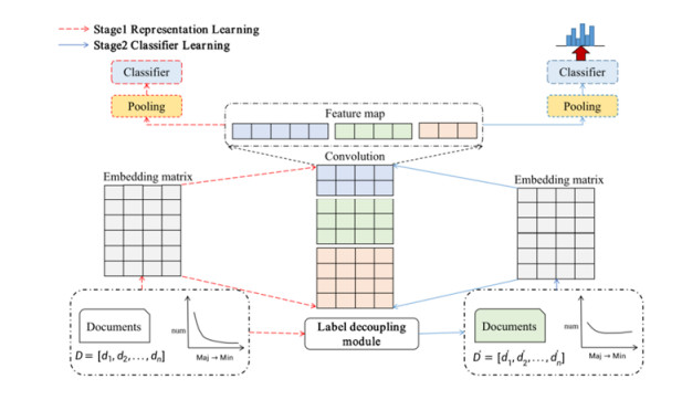
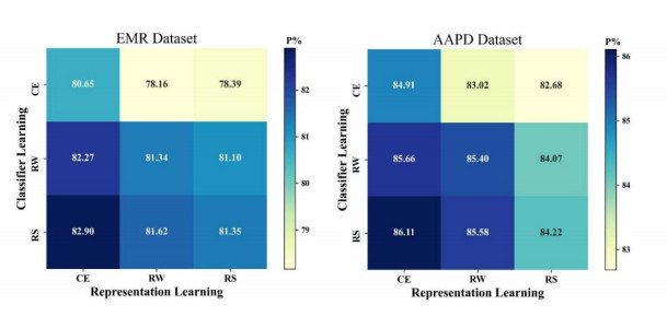
Electronic Medical Record (EMR) is the data basis of intelligent diagnosis. The diagnosis results of an EMR are multi-disease, including normal diagnosis, pathological diagnosis and complications, so intelligent diagnosis can be treated as multi-label classification problem. The distribution of diagnostic results in EMRs is imbalanced. And the diagnostic results in one EMR have a high coupling degree. The traditional rebalancing methods does not function effectively on highly coupled imbalanced datasets. This paper proposes Double Decoupled Network (DDN) based intelligent diagnosis model, which decouples representation learning and classifier learning. In the representation learning stage, Convolutional Neural Networks (CNN) is used to learn the original features of the data. In the classifier learning stage, a Decoupled and Rebalancing highly Imbalanced Labels (DRIL) algorithm is proposed to decouple the highly coupled diagnostic results and rebalance the datasets, and then the balanced datasets is used to train the classifier. This paper evaluates the proposed DDN using Chinese Obstetric EMR (COEMR) datasets, and verifies the effectiveness and universality of the model on two benchmark multi-label text classification datasets: Arxiv Academic Papers Datasets (AAPD) and Reuters Corpus1 (RCV1). Demonstrating the effectiveness of the proposed methods is an imbalanced obstetric EMRs. The accuracy of DDN model on COEMR, AAPD and RCV1 datasets is 84.17, 86.35 and 93.87% respectively, which is higher than the current optimal experimental results.
- imbalanced classification,
- decoupled,
- rebalancing methods,
- intelligent diagnosis
Citation: Kunli Zhang, Shuai Zhang, Yu Song, Linkun Cai, Bin Hu. Double decoupled network for imbalanced obstetric intelligent diagnosis[J]. Mathematical Biosciences and Engineering, 2022, 19(10): 10006-10021. doi: 10.3934/mbe.2022467

Related Papers:

Abstract

Electronic Medical Record (EMR) is the data basis of intelligent diagnosis. The diagnosis results of an EMR are multi-disease, including normal diagnosis, pathological diagnosis and complications, so intelligent diagnosis can be treated as multi-label classification problem. The distribution of diagnostic results in EMRs is imbalanced. And the diagnostic results in one EMR have a high coupling degree. The traditional rebalancing methods does not function effectively on highly coupled imbalanced datasets. This paper proposes Double Decoupled Network (DDN) based intelligent diagnosis model, which decouples representation learning and classifier learning. In the representation learning stage, Convolutional Neural Networks (CNN) is used to learn the original features of the data. In the classifier learning stage, a Decoupled and Rebalancing highly Imbalanced Labels (DRIL) algorithm is proposed to decouple the highly coupled diagnostic results and rebalance the datasets, and then the balanced datasets is used to train the classifier. This paper evaluates the proposed DDN using Chinese Obstetric EMR (COEMR) datasets, and verifies the effectiveness and universality of the model on two benchmark multi-label text classification datasets: Arxiv Academic Papers Datasets (AAPD) and Reuters Corpus1 (RCV1). Demonstrating the effectiveness of the proposed methods is an imbalanced obstetric EMRs. The accuracy of DDN model on COEMR, AAPD and RCV1 datasets is 84.17, 86.35 and 93.87% respectively, which is higher than the current optimal experimental results.

References

[1]	Y. Han, M. Tong, L. Jin, W. Meng, A. Ren, Maternal age at pregnancy and risk for gestational diabetes mellitus among Chinese women with singleton pregnancies, Int. J. Diabetes Dev. Countries, 41 (2021), 114–120. https://doi.org/10.1007/s13410-020-00859-8 doi: 10.1007/s13410-020-00859-8
[2]	K. Zhang, H. Ma, Y. Zhao, H. Zan, L. Zhuang, The comparative experimental study of multilabel classification for diagnosis assistant based on Chinese obstetric EMRs, J. Healthcare Eng., (2018), 1–9. https://doi.org/10.1155/2018/7273451 doi: 10.1155/2018/7273451
[3]	C. Xu, P. Liu, Y. Sun, Research on disease prediction model for unbalanced medical datasets, Chin. J. Comput., 42 (2019), 596–609. https://doi.org/10.11897/SP.J.1016.2019.00596 doi: 10.11897/SP.J.1016.2019.00596
[4]	Y. Liu, H. Loh, A. Sun, Imbalanced text classification: A term weighting approach, Expert Syst. Appl., 36 (2009), 690–701. https://doi.org/10.1016/j.eswa.2007.10.042 doi: 10.1016/j.eswa.2007.10.042
[5]	J. Stefanowski, Dealing with data difficulty factors while learning from imbalanced data, in Challenges in Computational Statistics and Data Mining, Springer, Cham, (2016), 333–363. https://doi.org/10.1007/978-3-319-18781-5_17
[6]	B. Zhou, Q. Cui, X. Wei, Z. Chen, BBN: Bilateral-branch network with cumulative learning for long-tailed visual recognition, in Proceedings of the IEEE/CVF Conference on Computer Vision and Pattern Recognition, (2020), 9719–9728. https://doi.org/10.1109/CVPR42600.2020.00974
[7]	B. Kang, S. Xie, M. Rohrbach, Z. Yan, A. Gordo, J. Feng, et al., Decoupling representation and classifier for long-tailed recognition, preprint, arXiv: 1910.09217.
[8]	Q. Yin, D. Shen, Y. Tang, Q. Ding, Intelligent monitoring of noxious stimulation during anaesthesia based on heart rate variability analysis, Comput. Biol. Med., 145 (2022), 105408. https://doi.org/10.1016/j.compbiomed.2022.105408 doi: 10.1016/j.compbiomed.2022.105408
[9]	T. Yan, P. Wong, C. Choi, C. Vong, H. Yu, Intelligent diagnosis of gastric intestinal metaplasia based on convolutional neural network and limited number of endoscopic images, Comput. Biol. Med., 126 (2020), 104026. https://doi.org/10.1016/j.compbiomed.2020.104026 doi: 10.1016/j.compbiomed.2020.104026
[10]	S. Wang, Y. Zhang, X. Cheng, X. Zhang, Y. Zhang, PSSPNN: PatchShuffle stochastic pooling neural network for an explainable diagnosis of COVID-19 with multiple-way data augmentation, Comput. Math. Methods Med., (2021), 1–18. https://doi.org/10.1155/2021/6633755 doi: 10.1155/2021/6633755
[11]	A. Rajkomar, E. Oren, K. Chen, A. Dai, N. Hajaj, M. Hardt, et al., Scalable and accurate deep learning with electronic health records, NPJ Digital Med., 1 (2018), 1–10. https://doi.org/10.1038/s41746-018-0029-1 doi: 10.1038/s41746-018-0029-1
[12]	A. Maxwell, R. Li, B. Yang, H. Weng, A. Ou, H. Hong, et al., Deep learning architectures for multi-label classification of intelligent health risk prediction, BMC. Bioinf., 18 (2017), 523. https://doi.org/10.1186/s12859-017-1898-z doi: 10.1186/s12859-017-1898-z
[13]	Z. Yang, Y. Huang, Y. Jiang, Y. Sun, Y. Zhang, P. Luo, et al., Clinical assistant diagnosis for electronic medical record based on convolutional neural network, Sci. Rep., 8 (2018), 6329. https://doi.org/10.1038/s41598-018-24389-w doi: 10.1038/s41598-018-24389-w
[14]	H. Liang, B. Tsui, H. Ni, C. Valentim, S. Baxter, G. Liu, et al., Evaluation and accurate diagnoses of pediatric diseases using artificial intelligence, Nat. Med., 25 (2019), 433. https://doi.org/10.1038/s41591-018-0335-9 doi: 10.1038/s41591-018-0335-9
[15]	N. Liu, E. Qi, M. Xu, B. Gao, G. Liu, A novel intelligent classification model for breast cancer diagnosis, Inf. Process. Manage., 56 (2019), 609–623. https://doi.org/10.1016/j.ipm.2018.10.014 doi: 10.1016/j.ipm.2018.10.014
[16]	C. Huang, X. Huang, Y. Fang, J. Xu, Y. Qu, P. Zhai, et al., Sample imbalance disease classification model based on association rule feature selection, Pattern Recognit. Lett., 133 (2020), 280–286. https://doi.org/10.1016/j.patrec.2020.03.016 doi: 10.1016/j.patrec.2020.03.016
[17]	B. Krawczyk, Learning from imbalanced data: Open challenges and future directions, Prog. Artif. Intell., 5 (2016), 221–232. https://doi.org/10.1007/s13748-016-0094-0 doi: 10.1007/s13748-016-0094-0
[18]	X. Liu, X. Sun, Y. Meng, J. Liang, F. Wu, J. Li, Dice loss for data-imbalanced NLP tasks, in Proceedings of the 58th Annual Meeting of the Association for Computational Linguistics, (2020), 465–476. https://doi.org/10.48550/arXiv.1911.02855
[19]	J. Yang, Z. Qu, Z. Liu, Improved feature-selection method considering the imbalance problem in text categorization, Sci. World J., (2014), 625342. https://doi.org/10.1155/2014/625342 doi: 10.1155/2014/625342
[20]	F. Charte, A. Rivera, M. Jesus, F. Herrera, A first approach to deal with imbalance in multi-label datasets, in International Conference on Hybrid Artificial Intelligence Systems, (2013), 150–160. https://doi.org/10.1007/978-3-642-40846-5_16
[21]	F. Charte, A. Rivera, M. Jesus, F. Herrera, Concurrence among imbalanced labels and its influence on multilabel resampling algorithms, in International Conference on Hybrid Artificial Intelligence Systems, (2014), 110–121. https://doi.org/10.1007/978-3-319-07617-1_10
[22]	F. Charte, A. Rivera, M. Jesus, F. Herrera, Resampling multilabel datasets by decoupling highly imbalanced labels, in International Conference on Hybrid Artificial Intelligence Systems, (2015), 489–501. https://doi.org/10.1007/978-3-319-19644-2_41
[23]	X. Glorot, Y. Bengio, Understanding the difficulty of training deep feedforward neural networks, in Proceedings of the Thirteenth International Conference on Artificial Intelligence and Statistics, JMLR Workshop and Conference Proceedings, (2010), 249–256. http://proceedings.mlr.press/v9/glorot10a
[24]	F. Charte, A. Rivera, M. Jesus, F. Herrera, Addressing imbalance in multilabel classification: Measures and random resampling algorithms, Neurocomputing, 163 (2015), 3–16. https://doi.org/10.1016/j.neucom.2014.08.091 doi: 10.1016/j.neucom.2014.08.091
[25]	D. Kingma, J. B. Adam, A method for stochastic optimization, preprint, arXiv: 1412.6980.
[26]	P. Yang, X. Sun, W. Li, S. Ma, W. Wu, H. Wang, SGM: Sequence generation model for multi-label classification, in Proceedings of the 27th COLING, (2018), 3915–3926. https://doi.org/10.48550/arXiv.1806.04822
[27]	D. Lewis, Y. Yang, T. Rose, F. Li, Rcv1: A new benchmark collection for text categorization research, Mach. Learn. Res., (2004), 361–397. https://research.gold.ac.uk/id/eprint/29758
[28]	M. Boutell, J. Luo, X. Shen, C. Brown, Learning multi-label scene classification, Pattern Recognit., 37 (2004), 1757–1771. https://doi.org/10.1016/j.patcog.2004.03.009 doi: 10.1016/j.patcog.2004.03.009
[29]	G. Tsoumakas, I. Katakis, Multi-label classification: An overview, Int. J. Data Warehous. Min., 3 (2007), 1–13. https://doi.org/10.4018/jdwm.2007070101 doi: 10.4018/jdwm.2007070101
[30]	Y. Chen, Convolutional neural networks for sentence classification, in Proceedings of 2014 Conference on Empirical Methods in Natural Language Processing (EMNLP), (2014), 1–62. http://hdl.handle.net/10012/9592

Reader Comments

Your name:*

Email:*
© 2022 the Author(s), licensee AIMS Press. This is an open access article distributed under the terms of the Creative Commons Attribution License (http://creativecommons.org/licenses/by/4.0)