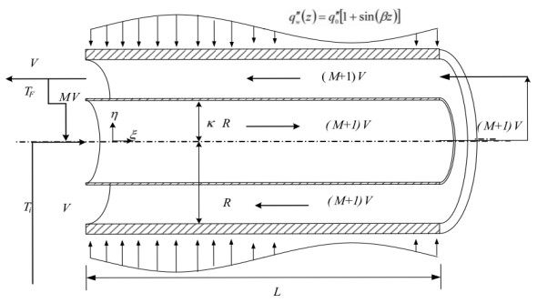
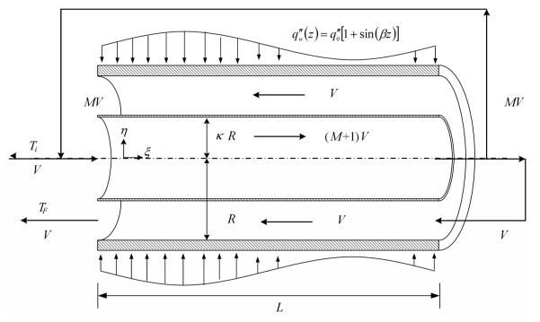
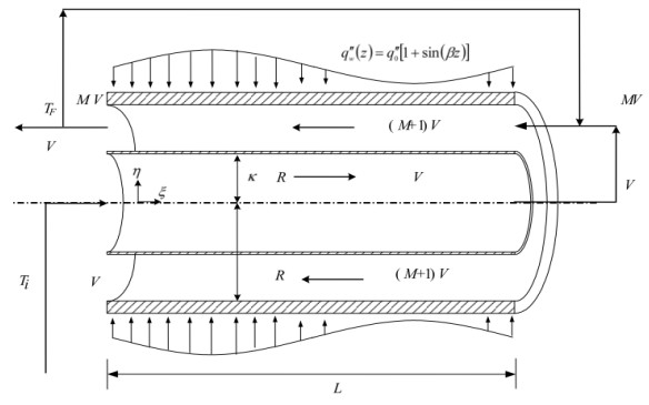
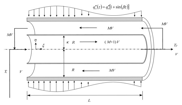
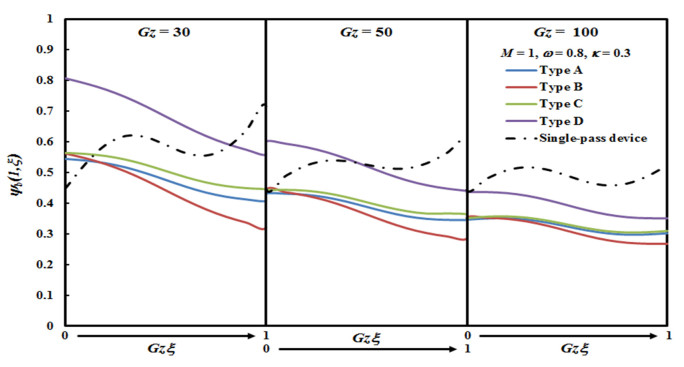
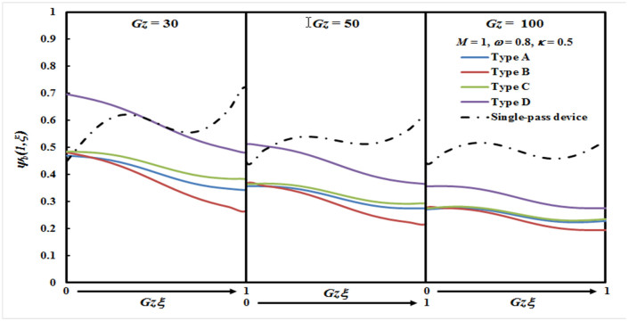
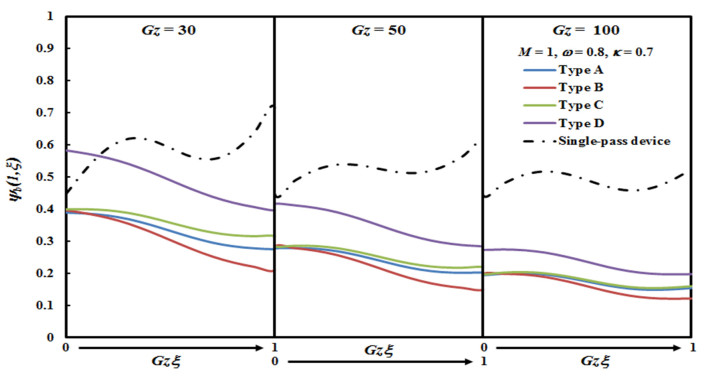
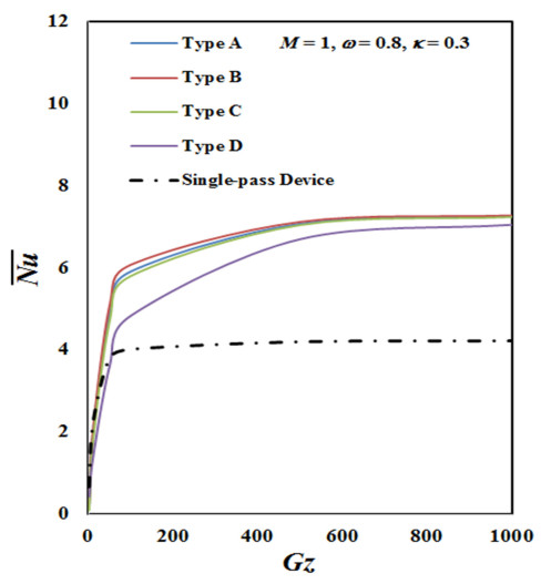
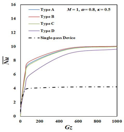
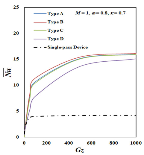
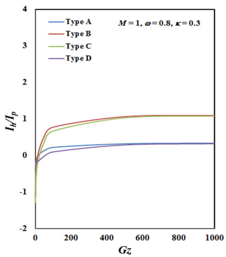
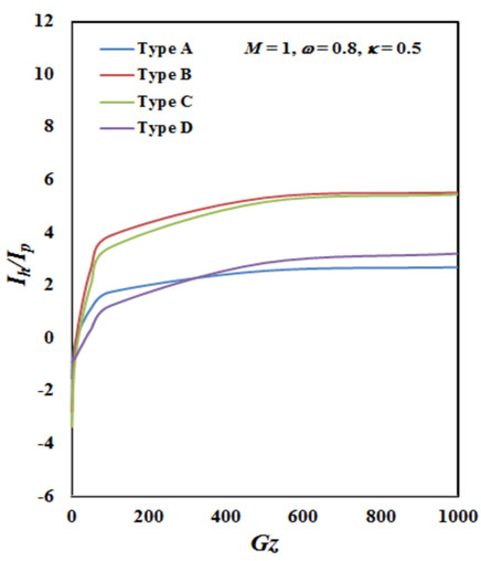
Effect of external-recycle operations on the heat-transfer efficiency, specifically for the power-law fluid flowing in double-pass concentric circular heat exchanger under sinusoidal wall fluxes, is investigated theoretically in the developed countries. Given that the fluid is heated twice on both sides of the impermeable sheet, four flow patterns proposed in recycling double-pass operations are expected to make substantial improvements in the performance of heat exchanger device in this study. Theoretical predictions point out that the heat-transfer efficiency increases with the ratio of channel thickness of double-pass concentric circular heat exchanger for all new designs under the same working dimension and the operational condition. The fluid velocity within the double-pass heat exchanger is increased by the fluids flowing through divided subchannels, which contributed to the higher convective heat-transfer efficiency. A simplified mathematical formulation was derived for double-pass concentric circular heat exchangers and would be a significant contribution to analyze heat transfer problems with sinusoidal wall fluxes at boundaries. The results deliver the optimal performance for the proposed four configurations with the use of external recycle compared to those conducted in single-pass, where an impermeable sheet is not inserted. The influences of power-law index and impermeable-sheet position on average Nusselt numbers under various flow patterns are also delineated. The distribution of dimensionless wall temperature was lower at the level of relative smaller thickness of annular channel, and the average Nusselt numbers for four external-recycle configurations and single-pass device were more suitable for operating under same condition. The ratio of the power consumption increment to heat-transfer efficiency enhancement demonstrates the economic feasibility among various configurations of double-pass concentric circular heat exchanger. The results also show that the external-recycle configuration (say Type B in the present study) serves as an important economic advantage in designing concentric circular heat exchangers for heating power-law fluids due to the smaller volumetric flow rate in annular channel with exiting outlet temperature.
Citation: Chii-Dong Ho, Jr-Wei Tu, Hsuan Chang, Li-Pang Lin, Thiam Leng Chew. Optimizing thermal efficiencies of power-law fluids in double-pass concentric circular heat exchangers with sinusoidal wall fluxes[J]. Mathematical Biosciences and Engineering, 2022, 19(9): 8648-8670. doi: 10.3934/mbe.2022401
Effect of external-recycle operations on the heat-transfer efficiency, specifically for the power-law fluid flowing in double-pass concentric circular heat exchanger under sinusoidal wall fluxes, is investigated theoretically in the developed countries. Given that the fluid is heated twice on both sides of the impermeable sheet, four flow patterns proposed in recycling double-pass operations are expected to make substantial improvements in the performance of heat exchanger device in this study. Theoretical predictions point out that the heat-transfer efficiency increases with the ratio of channel thickness of double-pass concentric circular heat exchanger for all new designs under the same working dimension and the operational condition. The fluid velocity within the double-pass heat exchanger is increased by the fluids flowing through divided subchannels, which contributed to the higher convective heat-transfer efficiency. A simplified mathematical formulation was derived for double-pass concentric circular heat exchangers and would be a significant contribution to analyze heat transfer problems with sinusoidal wall fluxes at boundaries. The results deliver the optimal performance for the proposed four configurations with the use of external recycle compared to those conducted in single-pass, where an impermeable sheet is not inserted. The influences of power-law index and impermeable-sheet position on average Nusselt numbers under various flow patterns are also delineated. The distribution of dimensionless wall temperature was lower at the level of relative smaller thickness of annular channel, and the average Nusselt numbers for four external-recycle configurations and single-pass device were more suitable for operating under same condition. The ratio of the power consumption increment to heat-transfer efficiency enhancement demonstrates the economic feasibility among various configurations of double-pass concentric circular heat exchanger. The results also show that the external-recycle configuration (say Type B in the present study) serves as an important economic advantage in designing concentric circular heat exchangers for heating power-law fluids due to the smaller volumetric flow rate in annular channel with exiting outlet temperature.

| [1] | R. K. Shah, A. L. London, Laminar Flow Forced Convection in Ducts, Academic Press, New York, U.S.A., (1978), 196-207. https://doi.org/10.1016/C2013-0-06152-X |
| [2] |
V. D. Dang, M. Steinberg, Convective diffusion with homogeneous and heterogeneous reaction in a tube, J. Phys. Chem., 84 (1980), 214-219. https://doi.org/10.1021/j100439a018 doi: 10.1021/j100439a018

|
| [3] |
E. Papoutsakis, D. Ramkrishna, Conjugated Graetz problems. I: General formalism and a class of solid-fluid problems, Chem. Eng. Sci., 36 (1981), 1381-1391. https://doi.org/10.1016/0009-2509(81)80172-8 doi: 10.1016/0009-2509(81)80172-8
|
| [4] |
X. Yin, H. H. Bau, The Conjugated Greatz problem with axial conduction, Trans. ASME, 118 (1996), 482-485. https://doi.org/10.1115/1.2825871 doi: 10.1115/1.2825871
|
| [5] |
D. Kaya, H. I. Sarac, Mathematical modeling of multiple-effect evaporators and energy economy, Energy, 32 (2007), 1536-1542. https://doi.org/10.1016/j.energy.2006.09.002 doi: 10.1016/j.energy.2006.09.002
|
| [6] |
J. Li, P. Hrnjak, Separation in condensers as a way to improve efficiency, Int. J. Refrig., 79 (2017), 1-9. https://doi.org/10.1016/j.ijrefrig.2017.03.017 doi: 10.1016/j.ijrefrig.2017.03.017
|
| [7] |
F. Reyes, W. L. Luyben, Extensions of the simultaneous design of gas-phase adiabatic tubular reactor systems with gas recycle, Ind. Eng. Chem. Res., 40 (2001), 635-647. https://doi.org/10.1021/ie000603j doi: 10.1021/ie000603j
|
| [8] |
C. M. C. Bonelli, A. F. Martins, E. B. Mano, C. L. Beatty, Effect of recycled polypropylene on polypropylene/high-density polyethylene blends, J. Appl. Polym. Sci., 80 (2001), 1305-1311. https://doi.org/10.1002/app.1217 doi: 10.1002/app.1217
|
| [9] |
M. A. Ebadian, H. Y. Zhang, An exact solution of extended Graetz problem with axial heat conduction, Int. J. Heat Mass Transfer, 32 (1989), 1709-1717. https://doi.org/10.1016/0017-9310(89)90053-7 doi: 10.1016/0017-9310(89)90053-7
|
| [10] |
C. Heinen, G. Guthausen, H. Buggisch, Determination of the power law exponent from magnetic resonance imaging (MRI) flow data, Chem. Eng. Technol., 25 (2002), 873-877. https://doi.org/10.1002/1521-4125(20020910)25:9 < 873::AID-CEAT873 > 3.0.CO; 2-T doi: 10.1002/1521-4125(20020910)25:9<873::AID-CEAT873>3.0.CO;2-T
|
| [11] |
R. P. Bharti, R. P. Chhabra, V. Eswaran, Steady forced convection heat transfer from a heated circular cylinder to power-law fluids, Int. J. Heat Mass Transfer, 50 (2007), 977-990. https://doi.org/10.1016/j.ijheatmasstransfer.2006.08.008 doi: 10.1016/j.ijheatmasstransfer.2006.08.008
|
| [12] |
A. Carezzato, M. R. Alcantara, J. Telis-Romero, C. C. Tadini, J. A. W. Gut, Non-Newtonian heat transfer on a plate heat exchanger with generalized configurations, Chem. Eng. Technol., 32 (2007), 21-26. https://doi.org/10.1002/ceat.200600294 doi: 10.1002/ceat.200600294
|
| [13] |
A. A. Delouei, M. Nazari, M. H. Kayhani, G. Ahmadi, Direct-forcing immersed boundary - non-Newtonian lattice Boltzmann method for transient non-isothermal sedimentation, J. Aerosol Sci., 104 (2017), 106-122. https://doi.org/10.1016/j.jaerosci.2016.09.002 doi: 10.1016/j.jaerosci.2016.09.002
|
| [14] |
A. A. Delouei, M. Nazari, M. H. Kayhani, G. Ahmadi, A non-Newtonian direct numeri-cal study for stationary and moving objects with various shapes: An immersed boundary - Lattice Boltzmann approach, J. Aerosol Sci., 93 (2016), 45-62. https://doi.org/10.1016/j.jaerosci.2015.11.006 doi: 10.1016/j.jaerosci.2015.11.006
|
| [15] |
A. A. Delouei, M. Nazari, M. H. Kayhani, S. Succi, Non-Newtonian unconfined flow and heat transfer over a heated cylinder using the direct-forcing immersed boundary-thermal la-ttice Boltzmann method, Phys. Rev. E, 89 (2014), 053312. https://doi.org/10.1103/PhysRevE.89.053312 doi: 10.1103/PhysRevE.89.053312
|
| [16] |
A. Jalali, A. A. Delouei, M. Khorashadizadeh, A. M. Golmohamadi, S. Karimnejad, Mesoscopic simulation of forced convective heat transfer of Carreau-Yasuda fluid flow over an inclined square: Temperature-dependent viscosity, J. Appl. Comput. Mech., 6 (2020), 307-319. https://doi.org/10.22055/JACM.2019.29503.1605 doi: 10.22055/JACM.2019.29503.1605
|
| [17] |
S. Aghakhani, A. H. Pordanjani, A. Karimipour, A. Abdollahi, M. Afrand, Numerical investigation of heat transfer in a power-law non-Newtonian fluid in a C-Shaped cavity with magnetic field effect using finite difference lattice Boltzmann method, Comput. Fluids, 176 (2018), 51-67. https://doi.org/10.1016/j.compfluid.2018.09.012 doi: 10.1016/j.compfluid.2018.09.012
|
| [18] |
J. M. Buick, Lattice Boltzmann simulation of power-law fluid flow in the mixing section of a single-screw extruder, Chem. Eng. Sci., 64 (2009), 52-58. https://doi.org/10.1016/j.ces.2008.09.016 doi: 10.1016/j.ces.2008.09.016
|
| [19] |
C. Y. Xie, J. Y. Zhang, V. Bertola, M. Wang, Lattice Boltzmann modeling for multiphase viscoplastic fluid flow, J. Non-Newtonian Fluid Mech., 234 (2016), 118-128. doi: 10.1016/j.jnnfm.2016.05.003
|
| [20] |
C. D. Ho, G. G. Lin, W. H. Lan, Analytical and experimental studies of power-law fluids in double-pass heat exchangers for improved device performance under uniform heat flu-xes, Int. J. Heat Mass Transfer, 61 (2013), 464-474. https://doi.org/10.1016/j.ijheatmasstransfer.2013.02.007 doi: 10.1016/j.ijheatmasstransfer.2013.02.007
|
| [21] |
S. Karimnejad, A. A. Delouei, M. Nazari, M. Shahmardan, A. Mohamad, Sedimentation of elliptical particles using Immersed Boundary-Lattice Boltzmann Method: A complementary repulsive force model, J. Mol. Liq., 262 (2018), 180-193. https://doi.org/10.1016/j.molliq.2018.04.075 doi: 10.1016/j.molliq.2018.04.075
|
| [22] |
S. Karimnejad, A. A. Delouei, M. Nazari, M. Shahmardan, M. Rashidi, S. Wongwises, Immersed boundary-thermal lattice Boltzmann method for the moving simulation of non-isothermal elliptical particles, J. Therm. Anal. Calorim., 138 (2019), 4003-4017. https://doi.org/10.1007/s10973-019-08329-y doi: 10.1007/s10973-019-08329-y
|
| [23] |
A. E. F. Monfared, A. Sarrafi, S. Jafari, M. Schaffie, Thermal flux simulations by lattice Boltzmann method; investigation of high Richardson number cross flows over tandem squa-re cylinders, Int. J. Heat Mass Transfer, 86 (2015), 563-580. https://doi.org/10.1016/j.ijheatmasstransfer.2015.03.011 doi: 10.1016/j.ijheatmasstransfer.2015.03.011
|
| [24] |
A. De Rosis, Harmonic oscillations of laminae in non-Newtonian fluids: a lattice Boltzmann-immersed boundary approach, Adv. Water Resour., 73 (2014), 97-107. https://doi.org/10.1016/j.advwatres.2014.07.004 doi: 10.1016/j.advwatres.2014.07.004
|
| [25] |
E. Aharonov, D. H. Rothman, Non-Newtonian flow (through porous media): A lattice-Boltzmann method, Geophys. Res. Lett., 20 (1993), 679-682. https://doi.org/10.1029/93GL00473 doi: 10.1029/93GL00473
|
| [26] |
A. Amiri Delouei, M. Nazari, M. Kayhani, S. Kang, S. Succi, Non-Newtonian particulate flow simulation: Adirect-forcing immersed boundary-lattice Boltzmann approach, Physica A, 447 (2016), 1-20. https://doi.org/10.1016/j.physa.2015.11.032 doi: 10.1016/j.physa.2015.11.032
|
| [27] |
C. J. Ho, W. C. Chen, W. M. Yan, M. Amani, Cooling performance of MEPCM suspensions for heat dissipation intensification in a minichannel heat sink, Int. J. Heat Mass Transfer, 115 (2017) 43-49. https://doi.org/10.1016/j.ijheatmasstransfer.2017.08.019 doi: 10.1016/j.ijheatmasstransfer.2017.08.019
|
| [28] |
C. J. Ho, P. C. Chang, W. M. Yan, P. Amani, Efficacy of divergent minichannels on cooling performance of heat sinks with water-based MEPCM suspensions, Int. J. Therm. Sci., 130 (2018) 333-346. https://doi.org/10.1016/j.ijthermalsci.2018.04.035 doi: 10.1016/j.ijthermalsci.2018.04.035
|
| [29] |
H. L. Tbena, M. I. Hasan, Numerical investigation of microchannel heat sink with MEPCM suspension with different types of PCM, Al-Qadisiyah J. Eng. Sci., 11 (2018), 115-133. https://doi.org/10.30772/qjes.v11i1.524 doi: 10.30772/qjes.v11i1.524
|
| [30] |
A. Sarı, C. Alkan, C. Bilgin, A. Bicer, Preparation, characterization and thermal energy storage properties of micro/nano encapsulated phase change material with acrylic-based polymer, Polym. Sci., Ser. B, 60 (2018), 58-68. https://doi.org/10.1134/S1560090418010128 doi: 10.1134/S1560090418010128
|
| [31] |
E. Alehosseini, S.M. Jafari, Micro/nano-encapsulated phase change materials (PCMs) as emerging materials for the food industry, Trends Food Sci. Technol., 91 (2019), 116-128. https://doi.org/10.1016/j.tifs.2019.07.003 doi: 10.1016/j.tifs.2019.07.003
|
| [32] |
M. Ghalambaz, J. Zhang, Conjugate solid-liquid phase change heat transfer in heatsink filled with phase change material-metal foam, Int. J. Heat Mass Transfer, 146 (2020), 118832-118849. https://doi.org/10.1016/j.ijheatmasstransfer.2019.118832 doi: 10.1016/j.ijheatmasstransfer.2019.118832
|
| [33] |
M. Ghalambaz, S. M. H. Zadeh, S. A. M. Mehryan, I. Pop, D. S. Wen, Analysis of melting behavior of PCMs in a cavity subject to a non-uniform magnetic field using a moving grid technique, Appl. Math. Model., 77 (2020), 1936-1953. https://doi.org/10.1016/j.apm.2019.09.015 doi: 10.1016/j.apm.2019.09.015
|
| [34] |
C. J. Ho, Y. C. Liu, M. Ghalambaz, W. M. Yan, Forced convection heat transfer of nano-encapsulated phase change material (NEPCM) suspension in a mini-channel heat sink, Int. J. Heat Mass Transfer, 155 (2020), 119858-119870. https://doi.org/10.1016/j.ijheatmasstransfer.2020.119858 doi: 10.1016/j.ijheatmasstransfer.2020.119858
|
| [35] |
S. A. M. Mehryan, L. S. Gargari, A. Hajjar, M. Sheremet, Natural convection flow of a suspension containing nano-encapsulated phase change particles in an eccentric annulus, J. Energy Storage, 28 (2020), 101236-101273. https://doi.org/10.1016/j.est.2020.101236 doi: 10.1016/j.est.2020.101236
|
| [36] |
J. F. Xie, B.Y. Cao, S. A. M. Mehryan, L. S. Gargari, A. Hajjar, M. Sheremet, Natural convection of power-law fluids under wall vibrations: A lattice Boltzmann study, Numer. Heat Transfer, Part A, 72 (2017), 600-627. https://doi.org/10.1080/10407782.2017.1394134 doi: 10.1080/10407782.2017.1394134
|
| [37] |
A. Petrovic, D. Lelea, I. Laza, The comparative analysis on using the NEPCM ma- terials and nanofluids for microchannel cooling solutions, Int. Commun. Heat Mass Transfer, 79 (2016), 39-45. https://doi.org/10.1016/j.icheatmasstransfer.2016.10.007 doi: 10.1016/j.icheatmasstransfer.2016.10.007
|
| [38] |
A. Hajjar, S. Mehryan, M. Ghalambaz, Time periodic natural convection heat transfer in a nano-encapsulated phase-change suspension, Int. J. Mech. Sci., 166 (2020) 105243. https://doi.org/10.1016/j.ijmecsci.2019.105243 doi: 10.1016/j.ijmecsci.2019.105243
|
| [39] |
M. Ghalambaz, T. Grosan, I. Pop, Mixed convection boundary layer flow and heat transfer over a vertical plate embedded in a porous medium filled with a suspension of nano-encapsulated phase change materials, J. Mol. Liq., 293 (2019), 111432. https://doi.org/10.1016/j.molliq.2019.111432 doi: 10.1016/j.molliq.2019.111432
|
| [40] |
V. D. Zimparov, A. K. da Silva, A. Bejan, Thermodynamic optimization of tree shaped flow geometries with constant channel wall temperature, Int. J. Heat Mass Transfer, 49 (2006), 4839-4849. https://doi.org/10.1016/j.ijheatmasstransfer.2006.05.024 doi: 10.1016/j.ijheatmasstransfer.2006.05.024
|
| [41] |
B. Weigand, D. Lauffer, The extended Graetz problem with piecewise constant wall temperature for pipe and channel flows, Int. J. Heat Mass Transfer, 47 (2004), 5303-5312. https://doi.org/10.1016/j.ijheatmasstransfer.2004.06.027 doi: 10.1016/j.ijheatmasstransfer.2004.06.027
|
| [42] |
A. Behzadmehr, N. Galanis, A. Laneville, Low Reynolds number mixed convection in vertical tubes with uniform wall heat flux, Int. J. Heat Mass Transfer, 46 (2003), 4823-4833. https://doi.org/10.1016/S0017-9310(03)00323-5 doi: 10.1016/S0017-9310(03)00323-5
|
| [43] |
O. Manca, S. Nardini, Experimental investigation on natural convection in horizontal channels with the upper wall at uniform heat flux, Int. J. Heat Mass Transfer, 50 (2007), 1075-1086. https://doi.org/10.1016/j.ijheatmasstransfer.2006.07.038 doi: 10.1016/j.ijheatmasstransfer.2006.07.038
|
| [44] |
C. J. Hsu, Heat transfer in a round tube with sinusoidal wall heat flux distribution, AIChE J., 11 (1965), 690-695. https://doi.org/10.1002/aic.690110423 doi: 10.1002/aic.690110423
|
| [45] |
A. Barletta, E. Rossi di Schio, Effects of viscous dissipation on laminar forced convection with axially periodic wall heat flux, Heat Mass Transfer, 35 (1999), 9-16. https://doi.org/10.1007/s002310050292 doi: 10.1007/s002310050292
|
| [46] |
D. K. Choi, D. H. Choi, Developing mixed convection flow in a horizontal tube under circumferentially non-uniform heating, Int. J. Heat Mass Transfer, 45 (1994), 1899-1913. https://doi.org/10.1016/0017-9310(94)90330-1 doi: 10.1016/0017-9310(94)90330-1
|
| [47] |
C. D. Ho, G. G. Lin, T. L. Chew, L. P. Lin, Conjugated heat transfer of power-law fluids in double-pass concentric circular heat exchangers with sinusoidal wall fluxes, Math. Biosci. Eng., 18 (2021), 5592-5613. https://doi.org/10.3934/mbe.2021282 doi: 10.3934/mbe.2021282
|
| [48] |
R. W. Hanks, K. M. Larsen, The flow of power-law non-Newtonian fluids in concentric annuli, Ind. Eng. Chem. Fundam., 18 (1979), 33-35. https://doi.org/10.1021/i160069a008 doi: 10.1021/i160069a008
|
| [49] |
D. Murkerjee, E. J. Davis, Direct-contact heat transfer immiscible fluid layers in laminar flow, AIChE J., 18 (1972), 94-101. https://doi.org/10.1002/aic.690180118 doi: 10.1002/aic.690180118
|
| [50] |
E. J. Davis, S. Venkatesh, The solution of conjugated multiphase heat and mass transfer problems, Chem. Eng. J., 34 (1979), 775-787. https://doi.org/10.1016/0009-2509(79)85133-7 doi: 10.1016/0009-2509(79)85133-7
|
| [51] |
A. Barletta, E. Zanchini, Laminar forced convection with sinusoidal wall heat flux distri-bution: axially periodic regime, Heat Mass Transfer, 31 (1995), 41-48. https://doi.org/10.1007/BF02537420 doi: 10.1007/BF02537420
|
| [52] | J. O. Wilkes, Fluid mechanics for chemical engineers, Prentice-Hall PTR, New Jersey, USA, 1999. |
| [53] | J. R. Welty, C. E. Wicks, R. E. Wilson, Fundamentals of Momentum, Heat, and Mass Transfer, John Wiley & Sons, New York, USA, 1984. |
Figures(13) / Tables(2)

Chii-Dong Ho, Jr-Wei Tu, Hsuan Chang, Li-Pang Lin, Thiam Leng Chew. Optimizing thermal efficiencies of power-law fluids in double-pass concentric circular heat exchangers with sinusoidal wall fluxes[J]. Mathematical Biosciences and Engineering, 2022, 19(9): 8648-8670. doi: 10.3934/mbe.2022401


 DownLoad: