Measuring the mobility impact on the COVID-19 pandemic

Thyago Celso C. Nepomuceno; Thalles Vitelli Garcez; Lúcio Camara e Silva; Artur Paiva Coutinho; Thyago Celso C. Nepomuceno; Thalles Vitelli Garcez; Lúcio Camara e Silva; Artur Paiva Coutinho

doi:10.3934/mbe.2022332

Mathematical Biosciences and Engineering

2022, Volume 19, Issue 7: 7032-7054. doi: 10.3934/mbe.2022332

Previous Article Next Article

Research article Special Issues

Measuring the mobility impact on the COVID-19 pandemic

1.
Núcleo de Tecnologia, Federal University of Pernambuco, Km 59, s/n, Nova Caruaru, Caruaru, PE, Brazil
2.
Dipartimento di Ingegneria Informatica Automatica e Gestionale Antonio Ruberti, Sapienza University of Rome, Via Ariosto, 25, Roma, Italy

Academic Editor: Daniel Rossit

Received: 28 December 2021 Revised: 11 April 2022 Accepted: 25 April 2022 Published: 12 May 2022

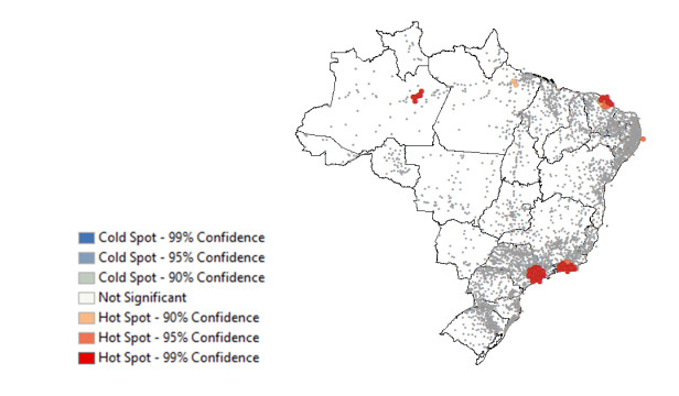
This assessment aims at measuring the impact of different location mobility on the COVID-19 pandemic. Data over time and over the 27 Brazilian federations in 5 regions provided by Google's COVID-19 community mobility reports and classified by place categories (retail and recreation, grocery and pharmacy, parks, transit stations, workplaces, and residences) are autoregressed on the COVID-19 incidence in Brazil using generalized linear regressions to measure the aggregate dynamic impact of mobility on each socioeconomic category. The work provides a novel multicriteria approach for selecting the most appropriate estimation model in the context of this application. Estimations for the time gap between contagion and data disclosure for public authorities' decision-making, estimations regarding the propagation rate, and the marginal mobility contribution for each place category are also provided. We report the pandemic evolution on the dimensions of cases and a geostatistical analysis evaluating the most critical cities in Brazil based on optimized hotspots with a brief discussion on the effects of population density and the carnival.

Keywords:

Citation: Thyago Celso C. Nepomuceno, Thalles Vitelli Garcez, Lúcio Camara e Silva, Artur Paiva Coutinho. Measuring the mobility impact on the COVID-19 pandemic[J]. Mathematical Biosciences and Engineering, 2022, 19(7): 7032-7054. doi: 10.3934/mbe.2022332

Related Papers:

[1]	Haiyan Wang, Nao Yamamoto . Using a partial differential equation with Google Mobility data to predict COVID-19 in Arizona. Mathematical Biosciences and Engineering, 2020, 17(5): 4891-4904. doi: 10.3934/mbe.2020266
[2]	Adil Yousif, Awad Ali . The impact of intervention strategies and prevention measurements for controlling COVID-19 outbreak in Saudi Arabia. Mathematical Biosciences and Engineering, 2020, 17(6): 8123-8137. doi: 10.3934/mbe.2020412
[3]	Lei Nie, Xin Guo, Chengqi Yi, Ruojia Wang . Analyzing the effects of public interventions on reducing public gatherings in China during the COVID-19 epidemic via mobile terminals positioning data. Mathematical Biosciences and Engineering, 2020, 17(5): 4875-4890. doi: 10.3934/mbe.2020265
[4]	Enahoro A. Iboi, Oluwaseun Sharomi, Calistus N. Ngonghala, Abba B. Gumel . Mathematical modeling and analysis of COVID-19 pandemic in Nigeria. Mathematical Biosciences and Engineering, 2020, 17(6): 7192-7220. doi: 10.3934/mbe.2020369
[5]	Fernando Saldaña, Hugo Flores-Arguedas, José Ariel Camacho-Gutiérrez, Ignacio Barradas . Modeling the transmission dynamics and the impact of the control interventions for the COVID-19 epidemic outbreak. Mathematical Biosciences and Engineering, 2020, 17(4): 4165-4183. doi: 10.3934/mbe.2020231
[6]	Fang Wang, Lianying Cao, Xiaoji Song . Mathematical modeling of mutated COVID-19 transmission with quarantine, isolation and vaccination. Mathematical Biosciences and Engineering, 2022, 19(8): 8035-8056. doi: 10.3934/mbe.2022376
[7]	M Kumaresan, M Senthil Kumar, Nehal Muthukumar . Analysis of mobility based COVID-19 epidemic model using Federated Multitask Learning. Mathematical Biosciences and Engineering, 2022, 19(10): 9983-10005. doi: 10.3934/mbe.2022466
[8]	Sarah R. Al-Dawsari, Khalaf S. Sultan . Modeling of daily confirmed Saudi COVID-19 cases using inverted exponential regression. Mathematical Biosciences and Engineering, 2021, 18(3): 2303-2330. doi: 10.3934/mbe.2021117
[9]	Wentao Hu, Yufeng Shi, Cuixia Chen, Ze Chen . Optimal strategic pandemic control: human mobility and travel restriction. Mathematical Biosciences and Engineering, 2021, 18(6): 9525-9562. doi: 10.3934/mbe.2021468
[10]	Hamed Karami, Pejman Sanaei, Alexandra Smirnova . Balancing mitigation strategies for viral outbreaks. Mathematical Biosciences and Engineering, 2024, 21(12): 7650-7687. doi: 10.3934/mbe.2024337

Abstract

1. Introduction

The current pandemic brought several uncertainties about social and economic prospects for many people due to public intervention policies ^[1]. Social distancing, lockdowns and quarantines became part of our daily base routines because they are assumed to be the most efficient non-pharmaceutical interventions (NPIs) to reduce the exponential tendency for any epidemic growth when vaccines are a scarce resource. Nevertheless, many disagreements on the matter of the mobility potential impact are still ignited by civil authorities over the world. While limiting people's mobility is a legit concern, especially justified by the economic downturns resulting from lockdowns, the lack of a solid argument and evidence counteract presidential speeches. However, they cannot prevent a biased public opinion on the subject.

Preventing jeopardizing health systems is undoubtedly the primary goal for any public authority resorting to quarantines and other measures reducing people's mobility. The current pandemic has ignited a response from the scientific community in basically all streams of research. Investigating the potential impact of different mobility dynamics is essential because public authorities' actions and studies on non-pharmaceutical interventions often include mobility sanctions as the primary strategy. Such measures include active case detection and isolation of infected persons, maintaining social distance, closure of schools and universities and most businesses, working from home when possible, quarantining and monitoring close contacts, and disclosure of multimedia epidemic and protection information by governments ^[2].

NPIs, including border restrictions, quarantine, social distancing, and changes in population behavior were associated with reduced transmission of COVID-19 in Hong Kong, and are also likely to have substantially reduced influenza transmission in early February 2020 ^[3]. Leung et al. ^[4] showed that the reproduction number (Rt) decreased substantially when control measures were implemented in all analyzed cities and provinces of China. In Brazil, Nepomuceno et al. ^[5,6] applied data envelopment analysis for healthcare performance assessment from two different perspectives considering hospital technical and human resources. The authors reported a positive association of the most inefficient Brazilian states in preventing infections (São Paulo, Bahia, Rio Grande do Sul and Paraná) with low rates of social isolation.

Brazil experienced peaks of 4211 and 4190 daily deaths on April 6 and April 8, 2021, and peaks of 115,041 daily cases (infections) on July 23, 2021 and 287,149 on February 3, 2022 (this last one resulted from the Omicron variant). Since June 2020, Brazil has been the second in the world in the number of COVID-19 deaths, above some of the most populated countries. One of the many reasons for the country's drastic situation is the recurrent position by the Federal Government downgrading the benefits of state-level mobility interventions. Brazil is perhaps the only big nation, in terms of geography, population or economy, that still has a leader maintaining a strong position against vaccines and the most commonly non-pharmaceutical measures. According to authors of Reference ^[7], who investigated geographic location data from 60 million mobile phones combined with voting information of 2018 national elections, social distancing and quarantines are significantly reduced in pro-government localities after Brazil's president dismissing the risks associated with the COVID-19 Pandemic, emphatically advising people to rebel against state mobility interventions.

Despite contrary and contradictory opinions by the federal government, most mobility sanctions and social distancing measures in Brazil started early, enforced by states and municipal authorities. From the third week of March 2020, many public policies were applied. Measures such as closing businesses, industries and services (considered non-essential), closing schools, universities and public places, gyms, theaters, cinemas, stadiums, limiting access to transport stations, and reinventing how typical workplaces operated. Nevertheless, except for very few moments in particular regions, the social isolation index has been beneath the expected. Brazil was declared the pandemic's emerging epicenter twice in May 2020 and March 2021, leading scholars to worry about a premature easing of restrictions effects on the number of COVID-19-related deaths ^[8].

The different interpretations of the current trade-off between economic development and the stability of the health systems can be attributed to a lack of feasible evaluations. From all the applied methodologies, generalized linear models (GLM) outstands among the approaches for determining associations of the COVID-19 and environmental, meteorological and ecological factors, including population density, temperature, solar radiation, air quality and meteorological variables ^{[9,10,11,12,13]}. Zhang et al. ^[14] employed a segmented Poisson model to analyze the available daily new cases data of the COVID-19 outbreaks in six countries, considering the governments' interventions (stay-at-home advises/orders, lockdowns, quarantines and social distancing). Another interesting instance is found in References ^[15,16], which investigated the contagion dynamics of the COVID-19 using a Poisson model autoregressed on daily new observed cases.

This work aims at evaluating the mobility impact on the pandemic over different mobility and socioeconomic categories. Section 2 is dedicated to details concerning the used dataset and the applied GLM and geostatistics methodologies. Sections 3–5 are reserved for the analysis, reporting how the most appropriate model was selected (based on a multiple criteria approach) and applied, discussing how the marginal contribution of each mobility category is coherent for the aggregate and first growth moments in Brazil. The spatial incidence in the most critical areas was investigated through optimized hot spots analysis in the fourth section, questioning some of the crisis's potential determinants and government responses. The conclusion summarizes the main findings and contributions of the model development and analysis.

2. Data and methods

During the first wave of COVID-19 in Brazil, especially in the first three months, the testing and data curation limitations lead the country to an average time lag of three weeks from the initial contamination until health authorities disclose information. This lag was because it took from one to two weeks to manifest the most severe symptoms that would lead a person to get tested for COVID-19, and from one to two weeks for the viral testing results. This empirical evidence had significant statistical support in our assessment when we performed a series of modeling considering time lags of 1, 2 and 3 weeks for new cases and total cases provided by Brazil (2020) ministry of health epidemiological report. We evaluated the percentage mobility in the six place categories offered by the google community mobility reports ^[17]: retail and recreation, grocery and pharmacy, parks, transit stations, workplaces, and residences. Georeferenced data at the federative level were obtained from Cota ^[18] COVID-19 repository.

The google mobility reports offer information on country and regions' movement trends over different place categories. The data reports how visits or time spent (in the case of residences) varies compared to a baseline proxy for what would represent a typical value for that day of the week. The baseline day is the median value from the five weeks from January 3 to February 6, 2020, which is appropriate for our study (first COVID-19 case in Brazil reported on February 26 and most mobility interventions took place from mid-March). Some locations composing the Parks category are gardens, castles, forests, campsites and observation decks. Some areas composing Transit Stations are seaports, taxi rank, metropolitan stations, car hire agencies and motorway services. Residences are measured in terms of duration percent changes instead of visit percent changes because this is where people spend much of the day. Box 1 presents all the variables considered in the analysis.

After the first crucial pandemic months, most regions observed more efficient testing and data curation. For this reason, the analysis for the aggregate mobility impact considering the entire 2020 was made on two weeks' time lag instead of three, which provided a more appropriate fitting for all potential model candidates with additive and multiplicative interactions, different probability distribution families (Gaussian, Gamma, Poisson) and link functions (identity, inverse and log).

Table Box 1. Variable definitions.

Infection Variables:

${\boldsymbol{Y}}_\mathbf{1}$ : New COVID-19 infections two weeks later;

${\boldsymbol{Y}}_\mathbf{2}$ : Total COVID-19 infections two weeks later;

${\boldsymbol{Y}}_\mathbf{1.3}$ : New COVID-19 infections three weeks later;

${\boldsymbol{Y}}_\mathbf{2.3}$ : Total COVID-19 infections three weeks later;

${\boldsymbol{y}}_\mathbf{1}$ : New COVID-19 infections in the same week of the mobility (two weeks before);

${\boldsymbol{y}}_\mathbf{2}$ : Total COVID-19 infections in the same week of the mobility (two weeks before);
Explanatory variables:

${\boldsymbol{x}}_\mathbf{1}$ : Mobility percent change in retail and recreation (from the baseline of February 2020);

${\boldsymbol{x}}_\mathbf{2}$ : Mobility percent change in grocery and pharmacy (from the baseline of February 2020);

${\boldsymbol{x}}_\mathbf{3}$ : Mobility percent change in parks (from the baseline of February 2020);

${\boldsymbol{x}}_\mathbf{4}$ : Mobility percent change in transit stations (from the baseline of February 2020);

${\boldsymbol{x}}_\mathbf{5}$ : Mobility percent change in workplaces (from the baseline of February 2020);

${\boldsymbol{x}}_\mathbf{6}$ : Mobility percent change in residential areas (from the baseline of February 2020);

${\boldsymbol{x}}_\mathbf{7}$ : Number of patients recovered
Interactions:

${{\boldsymbol{Y}}_\mathbf{1}\boldsymbol{x}}_\mathbf{1}$ ;

${{\boldsymbol{Y}}_\mathbf{1}\boldsymbol{x}}_\mathbf{2}$ ;

${{\boldsymbol{Y}}_\mathbf{1}\boldsymbol{x}}_\mathbf{3}$ ;

${{\boldsymbol{Y}}_\mathbf{1}\boldsymbol{x}}_\mathbf{4}$ ;

${{\boldsymbol{Y}}_\mathbf{1}\boldsymbol{x}}_\mathbf{5}$ ;

${{\boldsymbol{Y}}_\mathbf{1}\boldsymbol{x}}_\mathbf{6}$ : Interactions of new infections (2 weeks later) with the mobility;

${{\boldsymbol{Y}}_\mathbf{2}\boldsymbol{x}}_\mathbf{1}$ ;

${{\boldsymbol{Y}}_\mathbf{2}\boldsymbol{x}}_\mathbf{2}$ ;

${{\boldsymbol{Y}}_\mathbf{2}\boldsymbol{x}}_\mathbf{3}$ ;

${{\boldsymbol{Y}}_\mathbf{2}\boldsymbol{x}}_\mathbf{4}$ ;

${{\boldsymbol{Y}}_\mathbf{2}\boldsymbol{x}}_\mathbf{5}$ ;

${{\boldsymbol{Y}}_\mathbf{2}\boldsymbol{x}}_\mathbf{6}$ : Interactions of total infections (2 weeks later) with the mobility;

${{\boldsymbol{y}}_\mathbf{1}\boldsymbol{x}}_\mathbf{1}$ ;

${{\boldsymbol{y}}_\mathbf{1}\boldsymbol{x}}_\mathbf{2}$ ;

${{\boldsymbol{y}}_\mathbf{1}\boldsymbol{x}}_\mathbf{3}$ ;

${{\boldsymbol{y}}_\mathbf{1}\boldsymbol{x}}_\mathbf{4}$ ;

${{\boldsymbol{y}}_\mathbf{1}\boldsymbol{x}}_\mathbf{5}$ ;

${{\boldsymbol{y}}_\mathbf{1}\boldsymbol{x}}_\mathbf{6}$ : Interactions of new infections (2 weeks before) with the mobility;

${{\boldsymbol{y}}_\mathbf{2}\boldsymbol{x}}_\mathbf{1}$ ;

${{\boldsymbol{y}}_\mathbf{2}\boldsymbol{x}}_\mathbf{2}$ ;

${{\boldsymbol{y}}_\mathbf{2}\boldsymbol{x}}_\mathbf{3}$ ;

${{\boldsymbol{y}}_\mathbf{2}\boldsymbol{x}}_\mathbf{4}$ ;

${{\boldsymbol{y}}_\mathbf{2}\boldsymbol{x}}_\mathbf{5}$ ;

${{\boldsymbol{y}}_\mathbf{2}\boldsymbol{x}}_\mathbf{6}$ : Interactions of total infections (2 weeks before) with the mobility.

| Show Table

DownLoad: CSV

We have conducted two analyses for measuring the mobility impact on the number of infections: the first regarding the entire year, and the second, and more specific, for the beginning of the pandemic. The choice for the most appropriate models was based on statistical support, parsimony and quality of data/parameters to the empirical knowledge. Models of the Poisson family with log links presenting three weeks' time lag had a higher number of statistically significant variables and interactions (measured by the p-values) for the second analysis. Gaussian identity models with two weeks' time lag had the higher parsimony for the first analysis. Parsimony, measured by the Akaike information criterion (AIC) ^[19], refers to the trade-off between representativeness and simplicity of a model. The third criterion is an assumption based on specialized knowledge to avoid poor quality inputs. We have combined these perspectives into a multicriteria selection approach. This is explained in detail in Subsection 3.1 (model selection). General linear models with interactions sustained the best adherence to these criteria.

All daily-based data were aggregated per week by summing (the number of infections and recoveries) or taking the arithmetic average for the mobilities percent change. The boxplot visualizations of Figure 1 and the information in Table 1 summarize the main descriptive statistics. The x-axis assigns one box for each place category (retail and recreation, grocery and pharmacy, parks, transit stations, workplaces, and residences). The y-axis measures the minimum, first quartile, median, third quartile, maximum values, and outliers. Notches at the left and right sides of the median line are used to investigate potential differences in distributions' medians. When boxplots' notches overlap, there is some evidence that the medians are equal.

Figure 1. Boxplot visualizations for the mobility categories.

DownLoad: Full-Size Img PowerPoint

Table 1. Descriptive statistics.

Variable	Min.	1st Qu.	Median	Mean	3rd Qu.	Max.	Std. Dev.
${\boldsymbol{Y}}_\mathbf{1}$ : New infections	0.000	1336	4122	6794	8328	79,086	9068.515
${\boldsymbol{Y}}_\mathbf{2}$ : Total infections	0.000	9334	67,261	116,660	158,156	466,191	173,289.1
${\boldsymbol{x}}_\mathbf{1}$ : Retail and recreation	−81.29	−46.57	−26.86	−30.11	−15.00	13.71	20.742
${\boldsymbol{x}}_\mathbf{2}$ : Grocery and pharmacy	−47.86	−6.286	6.857	5.895	17.85	51.714	17.024
${\boldsymbol{x}}_\mathbf{3}$ : Parks	−82.43	−45.93	−27.50	−27.94	−11.18	36.50	23.191
${\boldsymbol{x}}_\mathbf{4}$ : Transit stations	−80.43	−49.29	−29.79	−28.85	−12.61	131.43	26.223
${\boldsymbol{x}}_\mathbf{5}$ : Workplaces	−58.85	−21.43	−95.000	−11.71	−0.428	208.571	15.473
${\boldsymbol{x}}_\mathbf{6}$ : Residential areas	−8.857	6.857	9.714	10.23	13.86	25.857	4.871
${\boldsymbol{x}}_\mathbf{7}$ : Recovery cases	0.000	2930	49,837	99,108	137,026	287,986	153,204.4

| Show Table

DownLoad: CSV

Autoregressive models with exogenous determinants are common for public policy, laws and sanctions evaluations ^[20]. Following a similar approach, and based on the decision criteria for choosing the most appropriate model, the number of new coronavirus infections is autoregressed to the number of new cases preceding 3 weeks and regressed to the interaction of COVID-19 base (the total number of cases up to the three weeks lag) with the place mobility variables for the analysis on the first growth. Formally:

$\mathrm{ln}{\lambda }_{i} = X\beta \therefore {y}_{i} = {e}^{X\beta }|{y}_{i}~Poisson\left({\lambda }_{i}\right)\forall i = 1, 2, 3, \dots , n$

(1)

where, $X\beta$ is the linear predictor ( ${b}_{0}+\prod _{j = 1}^{7}{b}_{j}{x}_{i}) \forall i = 1, 2, 3, \dots , n$ , with 120 multiplicative interactions, such that:

${b}_{0}$ = coefficient for the effect of COVID-19 new cases 3 reported weeks before (the R₀⁺)

${b}_{1}$ = coefficient for the effect of COVID-19 cases 3 reported weeks before (the R₀)

${b}_{2}$ = coefficient for the effect of retail and recreation mobility reported 3 weeks before

${b}_{3}$ = coefficient for the effect of grocery and pharmacy mobility reported 3 weeks before

${b}_{4}$ = coefficient for the effect of parks mobility reported 3 weeks before

${b}_{5}$ = coefficient for the effect of transit stations mobility reported 3 weeks before

${b}_{6}$ = coefficient for the effect of workplaces mobility reported 3 weeks before

${b}_{7}$ = coefficient for the effect of residences mobility reported 3 weeks before

Low mobility levels are expected to have a positive effect on reducing virus propagation considering the place categories. The log link function ( $ln {\lambda }_{i}$ ) in the Poisson GLM is appropriate in this modeling for keeping non-negative the projection λ when the mobility regressors X or coefficients β is expected to have negative values. Likewise, higher mobility is likely to contribute to increasing transmission.

The week from March 14 was considered the reference for counting the initial seed of cases. This is the week that 15 of the 27 federations disclosed the first cases, and most of\the state-level mobility sanctions were first implemented. The initial seed of cases works as a baseline to control the empirical estimation of the autoregressive covariate in this dynamic relationship. In addition, it works to identify the first week of significant macro data to model the phenomenon. Some federations have cases prior to the designed initial week. The northern states of Pernambuco (2 cases on March 12), Rio Grande do Norte (1 case on March 13), Alagoas (1 case on March 08) and Bahia (1 case on March 06) are some instances. The bigger seed of initial cases is for São Paulo, which had their first case on February 26, before any other federation, counting 56 new cases along the weeks until March 14, and 340 new cases in the first week from March 14, resulting in a seed of 396 initial cases.

3. Quantitative assessment

This section reports the results and discussion regarding the predictive modeling and marginal contributions of location mobility changes on different increasing or decreasing pandemic scenarios, considering an overall estimation for the country and additional regional assessments. First, we select the most appropriate econometric models by developing a multicriteria analysis considering the number of significant covariates using ROC weights for p-value intervals. Among the options, the choice is made over AIC ^[19] and empirical reasoning and vetoes imposed by multicollinearity testing. The mobility marginal contribution of each sector is then estimated in three pandemic scenarios for 2020 for each socioeconomic location at the state and national level.

3.1. Model selection

One of the primary goals in measuring the impact of some potential determinants on a dependent occurrence is selecting the most appropriate model based on identifying relevant independent (predictor) variables ^[21]. For this purpose, we set 40 generalized linear models with multiplicative interactions as potential candidates among many family distributions and link functions to explain the relationship between mobility in different locations and the pandemic outbreak. According to ^[22], the advantage of this approach is removing an unnecessarily restrictive assumption on a normally distributed error and the capacity to model different sorts of relations between the dependent variable and predictors. Among the models, we selected the 32 candidates that required less cognitive effort to explain the measure of marginal contribution for the mobility covariates (the impact of mobility on the COVID-19 spread).

On this set of 32 potential model candidates, we employed the multicriteria PROMETHEE (preference ranking organization method for enrichment evaluation) outranking ^[23] considering four significance intervals as criteria for the pairwise comparison: Criteria A: number of significant covariates with p-value varying in the interval from 0 to 0.001; Criteria B: number of significant covariates with p-value ranging in the interval from 0.001 to 0.01; Criteria C: number of significant covariates with p-value ranging in the interval from 0.01 to 0.05; and Criteria D: number of covariates with p-value ranging in the interval from 0.05 to 0.1. The PROMETHEE explores outranking relations by pairwise comparisons among models, and it provides a full rank of the candidates based on positive flows (score based on comparing models outranking other models) negative flows (score based on comparing models outranked by other models) and net flows (difference between positive and negative flows for a complete order).

One of the main issues in this process is how to define appropriate weights for the evaluation criteria (significant p-value intervals). The surrogate weighting procedure is the simplest method, not requiring additional cognitive efforts from a decision-maker. They come from predefined rankings converted into numerical weights by surrogate functions ^[24,25]. According to Almeida et al. ^[26], the surrogate weighting procedure more appropriate for the PROMETHEE procedure is the ROC (rank order centroid) method of Barron ^[27]. Compared to other methods, ROC weights attribute a more significant emphasis on the criteria ranked higher in the ranking construction, which is appropriate for our model selection since we consider more important the models with higher significant variables in explaining changes in the pandemic outbreak. Consider ${R}_{w} = \left\{{w}_{1}\ge {w}_{2}\ge {w}_{k}\ge \dots \ge {w}_{\mathrm{L}}\right\}$ a vector of weights for "k" models. The values for each rank position can be determined by:

${w}_{k} = \frac{1}{L}\sum _{\omega = k}^{L}\frac{1}{\omega }, k = \left\{\mathrm{1, 2}, \dots ., L\right\}$

(2)

From the 32 candidates, 16 have a positive net flow, which are ranked according to the AIC in Table 2. The BP p-value refers to the Breusch-Pagan test ^[28] for heteroskedasticity, considering the log transformation for the dependent variable. Because this multicriteria approach favors complex multivariate models, ranking the candidates based on AIC prevents a choice for an overfitting model, favoring the simplest yet most robust goodness of fit alternative. The first nine models are not significantly different in terms of AIC mean deviation. Despite a sizeable explanatory power, many models reported spurious correlations, multicollinearity, and aggregate data compensation bias (as defined by Nepomuceno and Costa ^[29]). For instance, models that considered the number of recovery cases reported a positive relation of this data regarding the spread of COVID-19 (models 17, 20, 21, 23 and 24), or some models reporting a negative association of the number of new cases (models 11 and 15) and total cases (model 4) with COVID-19 cases two weeks later (which would mean that more cases this week implies less propagation).

Table 2. Model candidates.

Criteria	A	B	C	D	Net Flow	AIC	BP P-value
ROC Weights	0.5208	0.2708	0.1458	0.0625	Net Flow	AIC	BP P-value
Model 2	7	0	0	0	0.1015	19,011.66	0.004306
Model 21	7	0	0	1	0.164	19,020.83	0.006528
Model 17	7	0	0	0	0.1015	19,021.72	0.004239
Model 24	8	0	0	0	0.3031	19,061.39	0.216777
Model 8	7	0	0	0	0.1015	19,068.6	0.137666
Model 20	7	0	0	0	0.1015	19,083.3	0.199999
Model 7	6	2	0	0	0.1653	19,188.64	0.053166
Model 1	7	0	0	1	0.164	19,220.5	0.006641
Model 23	6	1	1	1	0.2554	20,319.41	0.091411
Model 4	8	0	0	0	0.3031	22,260.87	0.000582
Model 18	7	1	0	0	0.3374	22,306.72	0.001029
Model 12	8	0	0	0	0.3031	23,548.04	0.0000152
Model 11	7	0	0	0	0.1015	25,899.05	0.009428
Model 13	7	1	0	0	0.3374	25,924.29	0.001113
Model 15	6	1	0	0	0.0517	26,996.51	0.002051
Model 9	6	1	0	0	0.0517	28,975.32	0.000189

| Show Table

DownLoad: CSV

The presence of multicollinearity means that two or more covariates are near perfect linear combinations of one another. It may imply in unstable or biased regression estimators, high standard errors or wide confidence intervals that may not reject the null hypothesis for the significance of variables, i.e., model parameters become indeterminate or problematic to estimate precisely. For testing multicollinearity in our models, we used variance inflation factor (VIF) diagnosis ^[30]. VIF measures how much variance is inflated from the expected true value due to correlations among the predictors. When VIF equals 1, no correlations among the predictors are observed. VIFs exceeding 10 indicate evidence of multicollinearity requiring correction ^[30].

The VIF is a veto for choosing the most appropriate candidate in the model selection. The most appropriate model was model 13, reporting minimum correlation among predictors. reports the VIFs and tolerance (variance percentage that cannot be accounted for by other predictors when the evaluated variable is regressed on the rest of the predictors in the model). illustrates the correlation matrix with a set of scattergrams between pairs of variables, excluding the variable ${Y}_{2}{x}_{1}$ reporting high multicollinearity.

Table 3. Multicollinearity diagnostic.

Variables	Description	Tolerance	VIF
${y}_{1}$	New COVID-19 infections in the same week of the mobility	0.14639	6.9870
${Y}_{2}{x}_{2}$	Interactions of infections (2 weeks later) with percent change mobilities on Groceries and Pharmacies	0.63853	1.5661
${Y}_{2}{x}_{3}$	Interactions of infections (2 weeks later) with percent change mobilities on Parks	0.30537	3.2747
${Y}_{2}{x}_{4}$	Interactions of infections (2 weeks later) with percent change mobilities on Transit Stations	0.12747	7.8446
${Y}_{2}{x}_{5}$	Interactions of infections (2 weeks later) with percent change mobilities on Workplaces	0.26626	3.7557
${Y}_{1}{x}_{6}$	Interactions of infections (2 weeks later) with percent change mobilities on Residences	0.24295	4.1161

| Show Table

DownLoad: CSV

Figure 2. Correlation matrix and dispersions.

DownLoad: Full-Size Img PowerPoint

3.2. Aggregate mobility impact

Each model candidate was checked considering the empirical reasoning reported in the previous subsection. The most appropriate model (Model 13) has seven very high significant variables (criteria A), the highest positive net flow of 0.3374 and AIC scoring 26,452.66. Retail and recreation reports a significant multicollinearity (VIF = 20.593403, tolerance = 0.04855924). For informational purposes, it is highlighted in red in the summary of Table 4. The model reports residual standard error (RSE) equal to 28,020 on 1127 degrees of freedom and Adjusted R-squared of 0.9739. Table 4 summarizes the model, residuals, covariates and other relevant statistics.

Table 4. Summary of results (aggregate impact).

Parameter	Marginal Contribution	Std. Error	p-value	Signf. Criteria	Mean (X)	Description
${\beta }_{0}$	1059.2	1086.3	0.33	Not significant	—	Intercept
${R}_{0}$	1.7355	0.246110	< 3.2e−12	Criteria A	86862.47	Marginal impact from the total COVID-19 Cases two weeks before ( ${y}_{2}$ )—the ${R}_{0}$ .
${\beta }_{1}$	−0.0178	0.000068	< 2e−16	Criteria A	−30.11235	Marginal impact from the interaction between cases and mobility in retail and recreation ( ${Y}_{2}\times {x}_{1}$ )
${\beta }_{2}$	0.03444	0.000328	< 2e−16	Criteria A	5.895083	Marginal impact from the interaction between cases and mobility in groceries and pharmacies ( ${Y}_{2}\times {x}_{2}$ )
${\beta }_{3}$	−0.00619	0.000300	< 2e−16	Criteria A	−27.93886	Marginal impact from the interaction between the cases and the mobility in parks two weeks before ( ${Y}_{2}\times {x}_{3}$ )
${\beta }_{4}$	−0.01366	0.000610	< 2e−16	Criteria A	−28.84866	Marginal impact from the interaction between cases and mobility in transit stations ( ${Y}_{2}\times {x}_{4}$ )
${\beta }_{5}$	−0.00929	0.000928	< 2e−16	Criteria A	−11.71315	Marginal impact from the interaction between cases and the mobility in workplaces ( ${Y}_{2}\times {x}_{5}$ )
${\beta }_{6}$	−0.06828	0.016185	2.63e−05	Criteria A	10.23406	Marginal impact from the interaction between cases and mobility in residences ( ${Y}_{2}\times {x}_{6}$ )
Note: Model 13: glm(formula = ${Y}_{2}$ ~ ${y}_{1}$ + ${Y}_{2}{x}_{2}$ + ${Y}_{2}{x}_{3}$ + ${Y}_{2}{x}_{4}$ + ${Y}_{2}{x}_{5}$ + ${Y}_{1}{x}_{6}$ ); Residuals: Min = −187800, 1^st Quartile = −9118, Median = −1165, 3^rdQuartile = 6739, Max = 210505; Residual standard error: 28020 on 1127 degrees of freedom; Multiple R-squared: 0.974; Adjusted R-squared: 0.9739; F-statistic: 7037 on 6 and 1127 DF; p-value: < 2.2e−16; AIC = 26452.66; PROMETHEE Net Flow = 0.3374; Min VIF = 1.566095 ( ${\beta }_{2})$ ; Max VIF = 7.844674 ( ${\beta }_{4}$ ).

| Show Table

DownLoad: CSV

The estimated model has good explanatory power with the intercept as the only not significant parameter. The autoregressive parameter (R₀) reporting 1.7355 means that, keeping all the mobility changes constant, 100 COVID-19 infections in the country two weeks before would produce about 173.55 new cases on average, with 99% confidence. Of course, this generalization does not consider individual regional characteristics, but it helps understand the complete panorama. According to the marginal contributions, the information about the mean of covariates reported in the sixth column helps interpret the relationship between the mobilities and COVID-19 cases. The mobility percentage change for retail and recreation, parks, transit stations and workplaces are negative for most of the year due to state-level mobility interventions and quarantine campaigns, which highly downward the overall mean to a negative value. For the mobility occurring in retail and recreation, one percent decrease in the negative mobility (one percent increase in mobility) provokes, on average, a positive response in the number of new COVID-19 cases in the amounts of 0.0178 $\times$ ${Y}_{2}$ . For instance, during the last week of September in the state of Ceará, this number would be 0.0178*4633 = 82.46 new cases, keeping everything else constant.

For the mobility occurring in parks, one percent increase in mobility (one percent decrease in the negative mobility) provokes, on average, a positive response of 0.00619 $\times$ ${Y}_{2}$ new COVID-19. For instance, during the second week of August in the state of Pernambuco, this estimate would be 0.00619 $\times$ 7537 = 46.65 new cases, keeping everything else constant. For the mobility occurring in transit stations, one percent decrease in the negative mobility (one percent increase in mobility) provokes, on average, a positive response in the number of new COVID-19 cases in the amounts of 0.01366 * ${Y}_{2}$ . For instance, during the last week of November in the state of Rio de Janeiro, this estimate would be 0.01366 $\times$ 20293 = 277.20 new cases, keeping everything else constant.

A slight (positive) change in mobility is observed for the groceries and pharmacies, which on average increased about 5.9% during the pandemic compared to one month before the first mobility restrictions. This can be attributed to the nature of those businesses (essential activities) which were not affected by the mobility sanctions and lockdowns. For the specific case of this mobility category, one percent increase in the mobility in groceries or pharmacies provokes, on average, a positive response in the number of COVID-19 new cases in the amounts of 0.000328 $\times$ ${Y}_{2}$ . For instance, during the first week of May in the state of São Paulo, this number would be 0.000328 $\times$ 11456 = 3.75 new cases, keeping everything else constant. During the last week of December in the state of Minas Gerais (one of the states with the best response to the pandemic in terms of mortality rate), this estimate would be 0.000328 $\times$ 26666 = 8.74 new cases, keeping everything else constant.

Increasing mobilities in workplaces provoke, on average, 0.00929 $\times$ ${Y}_{2}$ new cases. For the last example in Minas Gerais, this represent 0.00929 $\times$ 26666 = 247.72 new cases. Residential areas are the only mobility category reporting a negative relation with the number of COVID-19 new infections. The same relation was verified for the vast majority of models during the selection phase. The mobility change in residential areas is negative related to the number of new cases in the amount of -0.06828 $\times$ ${Y}_{2}$ . This estimate means that, in the examples of Ceará, São Paulo, Rio de Janeiro, Pernambuco and Minas Gerais, for every one percent increase in the mobility to residences, the number of COVID-19 cases would decrease in the amounts of 0.06828 $\times$ 4633 = 316.34, 0.06828 $\times$ 11456 = 782.21, 0.06828 $\times$ 20293 = 1385.60, 0.06828 $\times$ 7537 = 514.62 and 0.06828 $\times$ 26666 = 1820.75 cases, respectively.

3.3. Aggregate mobility impact on the first growth

Table 5 reports the main results for the mobility impact during the first pandemic growth. The coefficient sign represents the overall data relation of that specific base or place category with COVID-19 propagation (new cases). Two places categories exhibit a negative relation with COVID-19 (retail, recreation and workplaces). This can be interpreted as a spurious correlation problem: the same weeks an aggressive mobility reduction was observed in business, civic and cultural activities due to sanctions aiming at closing malls, shops, commercial centers, theaters, stadiums, outdoor events, service units and public administrations coincide with the COVID-19 exponential increase in Brazil. We cannot attribute, however, this increase to the mobility reduction in these places. This leads to believe correlation does not imply causation for these categories considering Brazil as a whole. This prospect may not be true for smaller disaggregated data on regions, states or municipalities.

Table 5. Estimates for Brazil on the first growth.

Covariates	Marginal contribution^{1, 2}	Exp. (Coeff.)	Coefficients	P-values	Signf. criteria
COVID-19 (R₀)	0.9026342	2.1831049	7.807e−01	< 2e−16	Criteria A
COVID-19 (R₀⁺)	7.49274	1.0020168	2.015e−03	< 2e−16	Criteria A
Retail & recreation	5.543848	0.1355574	−1.998e+00	< 2e−16	Criteria A
Grocery & pharmacy	−1.600595	19.7734385	2.984e + 00	< 2e−16	Criteria A
Parks	0.1696293	1.1263827	1.190e−01	0.01271	Criteria C
Transit stations	0.7903152	2.2323520	8.031e−01	4.03e−12	Criteria A
Workplaces	−3.774877	0.7883294	−2.378e−01	0.000103	Criteria A
Residences	3.760099	2.4628843	9.013e−01	0.000437	Criteria A
Note: glm(formula = ${Y}_{1}$ ~ ${b}_{0}+\prod _{j=1}^{7}{b}_{j}{x}_{i}$ ; Poisson (link = "log"); AIC: 14313; null dv.: 3229781 (173 df); res. dv.: 12680 (45 df); Fisher SI: 6; mult. interact. 120; min. dvrs.: −22.392; max. dvrs.: 34.825; 1q. dvrs.: −3.702; 3q. dvrs: 2.399; med. dvrs.: 0.018. ¹ Marginal contribution (Impact) in the cases from May 9 to May 16, 2020 (third week of May). ² Estimates for a marginal increment of one additional COVID-19 case and 0.001% additional mobility.

| Show Table

DownLoad: CSV

Another evidence is the exponential coefficient for these places categories. The exponential coefficient (Exp. Coeff.) is a proxy for how much new cases respond, on average, to cases and to mobility changes three weeks before. The estimates for retail and recreation and workplaces are small (0.135 and 0.788, respectively) compared to other estimates such as transit stations (2.232) and residences (2.463), despite the very significant p-values. The very high exponential coefficient for Grocery and Pharmacy is another instance of spurious data correlation in this case. The same weeks supermarkets, grocery stores and pharmacies have experienced a considerable demand increase coinciding with the COVID-19 exponential increase in Brazil. Nevertheless, we have no additional evidence to attribute COVID-19 exponential increase to the mobility increase in these places, leading to believe correlation does not imply causation for this category either, considering Brazil as a whole.

Because of the multiple interaction modeling structures, the exponential coefficients cannot be interpreted as additive predictors individually. Nevertheless, they provide a notion of the overall importance each base or place mobility has on new cases of COVID-19. We provide the marginal contribution estimates for a more empirical quantitative measure of the mobility impact. In this dynamic modeling, estimates for the R0, R0⁺ and for the mobility impact of each place category change along the time and along the regions and states. For each week and for each region, we have a different marginal contribution. The marginal contributions reported in Table 4 are estimations for the individual effect of each variable on the number of new coronavirus cases from May 9 to May 16, 2020. These are obtained by adding one unit change to the base of cases (new cases or total) or by adding 0.001% mobility change to the place category (retail and recreation, grocery and pharmacy, parks, transit stations, workplaces or residences), keeping everything else constant, them investigating the potential increase or decrease in the prediction for COVID-19. Statistical support is measured by the p-values.

Estimates for the R₀ and R₀⁺ vary according to the week and region. For the third week of May we can assume each new case three weeks before was responsible, on average, for 7.49 new cases. The mobility increase in grocery and pharmacy and workplaces had a negative effect on new cases, whereas the mobility increase in retail & recreation, parks, transit stations and residences had a positive effect. The positive effect of mobility changes in residential areas can be attributed to the vulnerability in favelas and poor communities. Despite the pandemic, Baile funk parties, peladas (pick-up soccer games) and many other forms of social organization are reported in many peripheries and informal urban settlements across the country.

The flexible scatterplots illustrate the mobility impact of each place category (retail and recreation, grocery and pharmacy, parks, transit stations, workplaces, residences) in the COVID-19 dissemination (new cases) in Brazil. They have different associations along the time depending on the number of confirmed cases (total). Taking the impact of retail and recreation as an example, the Poisson coefficient estimates an overall negative impact for this place category (see Table 5). However, the marginal contribution in the third week of May is positive because the number of cases 3 weeks before is 2167, and the retail and recreation mobility is between 60% and −40% (−57.66138 to be precise). This locates our estimation for the marginal contribution of retail and recreation mobility to the third frame of Figure 3 Panel (a), a positive effect of 5.5438 new cases for each 0.001% increase in mobility.

Figure 3. Dynamic mobility impact by place category in Brazil (first growth).

DownLoad: Full-Size Img PowerPoint

According to the different regions (north, northeast, center west, southeast and south), some estimates are reported in Tables 6–10. Figures 4–8 illustrate the spatial concentration. When disaggregating the country data into small datasets, there is a lack of significant samples for each region on the first growth. Therefore, most estimation for the mobility impact and contagion does not have statistical support. For this reason, this information is omitted in the Tables, only reporting the significant mobility impacts. The most significant impacts are the mobility in workplaces for the southeast region, parks for the center-west, residential areas in the northeast and retail and recreation in the north region. The estimates refer to a 1% marginal change in all categories.

Table 6. Estimates for the north region.

Covariates	Marginal contribution	P-value
COVID-19 (R₀)	3.981363	< 2e−16
Retail & recreation	635.1778	< 2e−16
Note: AIC: 2411; Poisson (link = "log"); null dev.: 74461.6 on 40 df.; res. Dev.: 2049.2 on 18 df; fisher SI: 5.

| Show Table

DownLoad: CSV

Table 7. Estimates for the northeast region.

Covariates	Marginal Contribution	P-value
COVID-19 (R₀)	0.7959314	< 2e−16
Retail & recreation	27.84628	< 2e−16
Parks	11.64888	< 2e−16
Workplaces	183.5822	< 2e−16
Residences	301.5848	< 2e−16
Note: AIC: 585.69; Poisson (link = "log"); null dev.: 1.054e+06 on 58 df.; res. dev.: 2.921e−12 on 0 df; fisher SI: 3.

| Show Table

DownLoad: CSV

Table 8. Estimates for the central-west region.

Covariates	Marginal Contribution	P-value
Parks	40.19183	0.0079
Note: AIC: 243.31; Poisson (link = "log"); null dev.: 7514.92 on 25 df.; res. dev.: 16.98 on 2 df; fisher SI: 4.

| Show Table

DownLoad: CSV

Table 9. Estimates for the southeast region.

Covariates	Marginal Contribution	P-value
COVID-19 (R₀)	—	—
COVID-19 (R₀⁺)	1.291627	< 2e−16 ***
Parks	9.183066	< 2e−16 ***
Workplaces	80.36371	< 2e−16 ***
Note: AIC: 655.84; Poisson (link = "log"); null dev.: 113107.42 on 27 df.; res. dev.: 351.29 on 4 df; fisher SI: 4.

| Show Table

DownLoad: CSV

Table 10. Estimates for the south region.

Covariates	Marginal contribution	P-value
No significant covariate

| Show Table

DownLoad: CSV

Figure 4. North.

DownLoad: Full-Size Img PowerPoint

Figure 5. Northeast.

DownLoad: Full-Size Img PowerPoint

Figure 6. Central west.

DownLoad: Full-Size Img PowerPoint

Figure 7. Southeast.

DownLoad: Full-Size Img PowerPoint

Figure 8. South.

DownLoad: Full-Size Img PowerPoint

4. Geospatial analysis

The most critical cities are evaluated using Optimized Hot Spots Analysis. This methodology offers statistics for each location indicating where cities with high or low COVID-19 cases cluster spatially ^[31]. The objective is to assess the COVID-19 intensity through cities. We question whether potential mobility contributions to eventual hot spots could indicate a spatial concentration of municipalities composing the input features aggregating the COVID-19 occurrences. A similar analysis can be accessed in References ^[29,32], investigating the spatial concentration of crime in Brazil's urban spaces. In this case, the occurrences for each geographic location are the analyzed field. Figure 9 presents the visualization.

Figure 9. COVID-19 Optimized hot spots in Brazil (first growth).

DownLoad: Full-Size Img PowerPoint

The hot spot cluster for 99% confidence is composed of the metropolitan areas of the capitals Manaus in the north, Ceará in the northeast, São Paulo and Rio de Janeiro in the southeast. In addition to significant COVID-19 incidence, these cities are surrounded by other cities with high COVID-19 incidence. These regions are the most probable responsible for the pandemic in the country. The impact on the health system is summed to a higher probability of contagion in these areas, which has made this significant spatial association critical and required urgent attention by the public authorities. Table 11 reports regional and aggregate descriptive typologies for additional insights in the spatial analysis. The feature input type is Brazil's municipalities (cities) containing COVID-19 infections per city as the analysis field. The number of valid inputs is 4965 with a maximum of 41451 infections in one single city in the southeast region, mean of 67.736, std. dev. equal to 781.06 and 66 outlier locations. The 99% confidence hot spots represent 6.76% of input features, highlighting the spatial concentration.

Table 11. Estimates and statistics for the spatial analysis.

Descriptive Statistics	North	Northeast	South	Southeast	Central West	Brazil
Cities	584	1898	787	1412	266	4965
Hotspots features*	41	79	75	175	11	336
Min. cases	1	1	1	1	1	1
Max. cases	12317	18644	711	41451	5542	41451
Total cases	65333	107939	14259	129531	9858	336311
Mean	111, 87	559.26	18.118	91.736	37.060	67.736
Std. dev.	651, 71	2385.2	62.635	225.67	345.75	781.062
Mean Z-score	0, 1227	0.0169	0.3124	0.2413	0.0684	0.0987
Std. dev. Z-score	1, 2170	1.1324	1.3373	1.4642	0.8758	1.38345
Mean P-value	0, 5200	0.6476	0.3767	0.6406	0.7292	0.62183
Std. dev. P-value	0, 2459	0.2574	0.3023	0.2592	0.2639	0.24533
Higher spatial concentration	Amazonas	Pernambuco; Ceará	Santa Catarina	São Paulo; Rio de Janeiro	Goiás; Distrito Federal	São Paulo; Rio de Janeiro
Note: At 99% confidence.*

| Show Table

DownLoad: CSV

The distances for geographic coordinates are analyzed using chordal distance in meters. Outliers were used to compute the optimal fixed distance band. There are 336 output features statistically significant based on false discovery rate correction for multiple testing and spatial dependence ^[33]. Figure 10 illustrates the distributions of optimized hot spots p-value frequencies, indicating the strength of spatial concentration per region. The p-values represent the statistical significance for whether or not to reject the null hypothesis that the observed high or low spatial clustering is different from a random distribution for the same features. High z-scores and small p-values for a feature indicate a spatial clustering of high COVID-19 infections. Low negative z-scores and small p-values indicate a spatial clustering of low COVID-19 cases. Higher p-values indicate no significant spatial clustering. The region with smaller p-value distributions (below 0.05) is the South, reporting an average 0.3767 p-value.

Figure 10. P-value frequency distributions.

DownLoad: Full-Size Img PowerPoint

We can see the regions reporting the most significant hot spots (north, northeast and southeast) undergo unregular frequency distributions, basically concentrating the pandemic in singular features. Some potential explanations are discussed ahead. Rio de Janeiro and São Paulo states have the second and third highest population density, and they have the fifth and second capitals with the highest population density. Ceará has the capital with the highest population density in Brazil. This information, combined with the airline hubs for international flights in these capitals, can explain, at least partially, the high initial incidence and fast spread of COVID-19.

Another factor that may explain the critical scenario for those regions is related to the most famous Brazilian festival: the carnival. Table 12 reports the average percentage mobility 3 weeks prior to the first confirmed cases of community Transmission on each state in the hot spot cluster. Community transmission is characterized when authorities are unable to trace the source of the infection. The states of São Paulo (SP) and Rio de Janeiro (RJ) have the first community transmission officially reported on March 13. According to our specifications, the first case can be traced back to the last week of February during the carnival holidays. During the carnival week, all place categories in São Paulo and Rio de Janeiro had a negative mobility change, with an exemption on parks and residential areas which are the places concentrating street carnival and parades.

Table 12. Average mobility (3 weeks prior to the first to community transmission).

UF	Week n-3	Retail & Recreation	Grocery & Pharmacy	Parks	Transit stations	Workplaces	Residences
SP	4th Feb. (carnival)	−9571	−1857	6286	−11,286	−12,571	4429
RJ	4th Feb. (carnival)	−13,857	−5714	32,286	−11,000	−27,143	5429
CE	1st March	−9571	1714	−29,571	−2,857	8143	1571
AM	2nd March	2286	6857	1000	15,000	15,143	−1429

| Show Table

DownLoad: CSV

5. Conclusions

Brazil's COVID-19 response has been one of the most controversial in the world. If, on one hand, state governments and municipalities' efforts follow international protocols and recommendations, on the other, there is a big question about the federal administration's institutional preparedness, which constantly jeopardizes the prospects of mobility sanctions, social distancing, and quarantine campaigns. The results reported in this assessment aim at contributing to this discussion. In particular, reducing mobility in residential areas and retail places is a challenge local authorities should prioritize due to their high potential. Non-parametric governance models for prioritizing and allocating resources and benchmarking knowledge from local administrations with efficient mobility strategies can be an interesting avenue ^[34,35,36]. The absence of the state in favelas can make longer the trade-off between the economy and health. Unquarantine planning based on the individual impact of these place categories and the interaction with external localities can anticipate optimal responses for Brazilian communities to prevent drastic outcomes from the pandemic. For a more profound knowledge on this topic, please refer to this reference list with recent applications in Brazil ^{[37,38,39,40,41,42,43,44,45,46,47,48,49,50,51,52,53,54,55]}.

Acknowledgement

The authors acknowledge the support from the Federal University of Pernambuco through the called "Edital Propesq nº 06/2020 – Edital Emergencial de Credenciamento e Fomento de Projetos, Visando Ações para o Diagnóstico e Prevenção da Covid-19".

Conflict of interest

Authors declare no conflict of interest.

References

[1]	G. Caggiano, E. Castelnuovo, R. Kima, The global effects of COVID-19-induced uncertainty, Econ. Lett., 194 (2020), 109392. https://doi.org/10.1016/j.econlet.2020.109392 doi: 10.1016/j.econlet.2020.109392
[2]	J. Sun, Z. Shi, H. Xu, Non-pharmaceutical interventions used for COVID-19 had a major impact on reducing influenza in China in 2020, J. Travel Med., 27 (2020), taaa064. https://doi.org/10.1093/jtm/taaa064 doi: 10.1093/jtm/taaa064
[3]	C. M. Herren, T. K. Brownwright, E. Y. Liu, N. E. Amiri, M. Majumder, Democracy and mobility: a preliminary analysis of global adherence to non-pharmaceutical interventions for COVID-19, Soc. Sci. Res. Network, 2020 (2020). https://doi.org/10.2139/ssrn.3570206
[4]	K. Leung, J. T. Wu, D. Liu, G. M. Leung, First-wave COVID-19 transmissibility and severity in China outside Hubei after control measures, and second-wave scenario planning: a modelling impact assessment, Lancet, 395 (2020), 1382–1393. https://doi.org/10.1016/S0140-6736(20)30746-7 doi: 10.1016/S0140-6736(20)30746-7
[5]	T. C. C. Nepomuceno, W. M. N. Silva, K. T. C. Nepomuceno, I. K. F. Barros, A DEA-based complexity of needs approach for hospital beds evacuation during the COVID-19 outbreak, J. Healthcare Eng., 2020 (2020). https://doi.org/10.1155/2020/8857553
[6]	T. C. C. Nepomuceno, W. M. N. Silva, S. D. F. Gomes, T. F. O. Rodriguez, Comparative network efficiency analysis of Brazil response to COVID-19 at state level, Value Health, 24 (2021), S175. https://doi.org/10.1016/j.jval.2021.04.868 doi: 10.1016/j.jval.2021.04.868
[7]	N. Ajzenman, T. Cavalcanti, D. da Mata, More than words: leaders' speech and risky behavior during a pandemic, preprint. https://dx.doi.org/10.2139/ssrn.3582908
[8]	M. B. Neiva, I. Carvalho, E. D. S. Costa, F. Barbosa-Junior, F. A. Bernardi, T. L. M. Sanches, et al., Brazil: the emerging epicenter of COVID-19 pandemic, Rev. Soc. Bras. Med. Trop., 53 (2020). https://doi.org/10.1590/0037-8682-0550-2020 doi: 10.1590/0037-8682-0550-2020
[9]	H. Xu, C. Yan, Q. Fu, K. Xiao, Y. Yu, D. Han, et al., Possible environmental effects on the spread of COVID-19 in China, Sci. Total Environ., 731 (2020), 139211. https://doi.org/10.1016/j.scitotenv.2020.139211 doi: 10.1016/j.scitotenv.2020.139211
[10]	P. Byass, Eco-epidemiological assessment of the COVID-19 epidemic in China, January–February 2020, Global Health Action, 13 (2020), 1760490. https://doi.org/10.1080/16549716.2020.1760490 doi: 10.1080/16549716.2020.1760490
[11]	M. Ujiie, S. Tsuzuki, N. Ohmagari, Effect of temperature on the infectivity of COVID-19, Int. J. Infect. Dis., 95 (2020), 301–303. https://doi.org/10.1016/j.ijid.2020.04.068 doi: 10.1016/j.ijid.2020.04.068
[12]	Y. Jiang, X. J. Wu, Y. J. Guan, Effect of ambient air pollutants and meteorological variables on COVID-19 incidence, Infect. Control Hosp. Epidemiol., 41 (2020), 1011–1015. https://doi.org/10.1017/ice.2020.222 doi: 10.1017/ice.2020.222
[13]	A. Altamimi, A. E. Ahmed, Climate factors and incidence of Middle East respiratory syndrome coronavirus, J. Infect. Public Health, 13 (2019), 704–708. https://doi.org/10.1016/j.jiph.2019.11.011. doi: 10.1016/j.jiph.2019.11.011
[14]	X. Zhang, R. Ma, L. Wang, Predicting turning point, duration and attack rate of COVID-19 outbreaks in major western countries, Chaos Solitons Fractals, 135 (2020), 109829. https://doi.org/10.1016/j.chaos.2020.109829 doi: 10.1016/j.chaos.2020.109829
[15]	A. Agosto, P. Giudici, A poisson autoregressive model to underaimstand COVID-19 contagion dynamics, Risks, 8 (2020), 77. https://doi.org/10.3390/risks8030077 doi: 10.3390/risks8030077
[16]	A. Agosto, P. Giudici, COVID-19 contagion and digital finance, Digital Finance, 2 (2020), 159–167. https://doi.org/10.1007/s42521-020-00021-3 doi: 10.1007/s42521-020-00021-3
[17]	Google LLC, Google COVID-19 Community Mobility Reports. Available from: https://www.google.com/covid19/mobility/.
[18]	W. Cota, Monitoring the number of COVID-19 cases and deaths in brazil at municipal and federative units level, preprint. https://orcid.org/0000-0002-8582-1531
[19]	H. Akaike, A new look at the statistical model identification, IEEE Trans. Autom. Control, 19 (1974), 716–723. https://doi.org/10.1109/TAC.1974.1100705 doi: 10.1109/TAC.1974.1100705
[20]	T. C. C. Nepomuceno, J. A. de Moura, L. C. e Silva, A. P. C. S. Costa, Alcohol and violent behavior among football spectators: An empirical assessment of Brazilian's criminalization, Int. J. Law, Crime Justice, 51 (2017), 34–44. https://doi.org/10.1016/j.ijlcj.2017.05.001 doi: 10.1016/j.ijlcj.2017.05.001
[21]	R. S. Halinski, L. S. Feldt, The selection of variables in multiple regression analysis, J. Educ. Meas., 7 (1970), 151–157. https://doi.org/10.1111/j.1745-3984.1970.tb00709.x doi: 10.1111/j.1745-3984.1970.tb00709.x
[22]	F. A. van Eeuwijk, Multiplicative interaction in generalized linear models, Biometrics, 51 (1995), 1017–1032. https://doi.org/10.2307/2533001 doi: 10.2307/2533001
[23]	J. P. Brans, P. Vincke, A preference ranking organization method, Manage. Sci., 31 (1985), 647–656. https://doi.org/10.1287/mnsc.31.6.647 doi: 10.1287/mnsc.31.6.647
[24]	F. H. Barron, B. E. Barrett, Decision quality using ranked attribute weights, Manag. Sci., 42 (1996), 1515–1523. https://doi.org/10.1287/mnsc.42.11.1515 doi: 10.1287/mnsc.42.11.1515
[25]	M. Danielson, L. Ekenberg, Trade-offs for ordinal ranking methods in multicriteria decisions, in International Conference on Group Decision and Negotiation, (2016), 16–27. https://doi.org/10.1007/978-3-319-52624-9_2
[26]	A. T. de Almeida Filho, T. R. N. Clemente, M. D. Costa, A. T. Almeida, Preference modeling experiments with surrogate weighting procedures for the PROMETHEE method, Eur. J. Oper. Res., 264 (2018), 453–461. https://doi.org/10.1016/j.ejor.2017.08.006 doi: 10.1016/j.ejor.2017.08.006
[27]	F. H. Barron, Selecting a best multi-attribute alternative with partial information about attribute weights, Acta Psychol., 80 (1992), 91–103. https://doi.org/10.1016/0001-6918(92)90042-C doi: 10.1016/0001-6918(92)90042-C
[28]	T. S. Breusch, A. R. Pagan, A simple test for heteroscedasticity and random coefficient variation, Econometrica J. Econometric Soc., (1979), 1287–1294. https://doi.org/10.2307/1911963
[29]	T. C. C. Nepomuceno, A. P. C. S.Costa, Spatial visualization on patterns of disaggregate robberies, Oper. Res. Int. J., 19 (2019), 857–886. https://doi.org/10.1007/s12351-019-00479-z doi: 10.1007/s12351-019-00479-z
[30]	D. A. Belsley, E. Kuh, R. E. Welsch, Regression Diagnostics: Identifying Influential Data and Sources of Collinearity, John Wiley & Sons, New York, 1980.
[31]	A. Getis, J. K. Ord, The analysis of spatial association by use of distance statistics, Geogr. Anal., 24 (1992), 189–206. https://doi.org/10.1111/j.1538-4632.1992.tb00261.x doi: 10.1111/j.1538-4632.1992.tb00261.x
[32]	T. Menezes, R. Silveira-Neto, C. Monteiro, J. L. Ratton, Spatial correlation between homicide rates and inequality: evidence from urban neighborhoods, Econ. Lett., 120 (2013), 97–99. https://doi.org/10.1016/j.econlet.2013.03.040. doi: 10.1016/j.econlet.2013.03.040
[33]	Y. Benjamini, Y. Hochberg, Controlling the false discovery rate: a practical and powerful approach to multiple testing, J. R. Stat. Soc. B, 57 (1995), 289–300. https://doi.org/10.1111/j.2517-6161.1995.tb02031.x doi: 10.1111/j.2517-6161.1995.tb02031.x
[34]	T. C. C. Nepomuceno, A. P. C. Costa, Resource allocation with time series DEA applied to Brazilian federal saving banks, Econ. Bull., 39 (2019), 1384–1392.
[35]	T. C. C. Nepomuceno, V. D. H. De Carvalho, A. P. C. S. Costa, Time-series directional efficiency for knowledge benchmarking in service organizations, iin World Conference on Information Systems and Technologies, 2020. https://doi.org/10.1007/978-3-030-45688-7_34
[36]	T. C. C. Nepomuceno, V. D. H. de Carvalho, K. T. C. Nepomuceno, A. P. C. S. Costa, Exploring knowledge benchmarking using time‐series directional distance functions and bibliometrics, Exp. Syst., 2022 (2022), e12967. https://doi.org/10.1111/exsy.12967 doi: 10.1111/exsy.12967
[37]	M. Fiori, G. Bello, N. Wschebor, F. Lecumberry, A. Ferragut, E. Mordecki, Decoupling between SARS-CoV-2 transmissibility and population mobility associated with increasing immunity from vaccination and infection in south America, Sci. Rep., 12 (2022), 1–9. https://doi.org/10.1038/s41598-022-10896-4 doi: 10.1038/s41598-022-10896-4
[38]	B. R. G. M. Couto, J. J. da Cunha Junior, C. D. M. Oliveira, H. D. D. de Carvalho, Rhayssa F. A. Rocha, A. L. Alvim, et al., Mobility restrictions for the control of COVID-19 epidemic, preprints. https://doi.org/10.1590/SciELOPreprints.717
[39]	P. J. Puccinelli, T. S. da Costa, A. Seffrin, C. A. B. de Lira, R. L. Vancini, P. T. Nikolaidis, et al., Correction to: reduced level of physical activity during COVID-19 pandemic is associated with depression and anxiety levels: an internet-based survey, BMC Public Health, 21 (2021), 1–11. https://doi.org/10.1186/s12889-021-10684-1 doi: 10.1186/s12889-021-10684-1
[40]	P. J. Pérez-Martínez, J. A. Dunck, J. V. de Assunção, P. Connerton, A. D. Slovic, H. Ribeiro, et al., Long-term commuting times and air quality relationship to COVID-19 in São Paulo, J. Transp. Geogr., 2022 (2022), 103349. https://doi.org/10.1016/j.jtrangeo.2022.103349 doi: 10.1016/j.jtrangeo.2022.103349
[41]	A. P. Rudke, D. S. de Almeida, R. A. Alves, A. Beal, L. D. Martins, J. A. Martins, et al., Impacts of strategic mobility restrictions policies during 2020 COVID-19 outbreak on Brazil's regional air quality, Aerosol Air Qual. Res., 22 (2022), 210351. https://doi.org/10.4209/aaqr.210351 doi: 10.4209/aaqr.210351
[42]	C. S. Costa, C. S. Pitombo, F. L. U. D. Souza, Travel behavior before and during the COVID-19 pandemic in Brazil: mobility changes and transport policies for a sustainable transportation system in the post-pandemic period, Sustainability, 14 (2022), 4573. https://doi.org/10.3390/su14084573 doi: 10.3390/su14084573
[43]	L. Ferrante, L. H. Duczmal, E. Capanema, W. A. C. Steinmetz, A. C. L. Almeida, J. Leão, et al., Dynamics of COVID-19 in Amazonia: a history of government denialism and the risk of a third wave, Prev. Med. Rep., 26 (2022), 101752. https://doi.org/10.1016/j.pmedr.2022.101752 doi: 10.1016/j.pmedr.2022.101752
[44]	S. Ibarra-Espinosa, E. D. de Freitas, K. Ropkins, F. Dominici, A. Rehbein, Negative-binomial and quasi-poisson regressions between COVID-19, mobility and environment in São Paulo, Brazil, Environ. Res., 204 (2022), 112369. https://doi.org/10.1016/j.envres.2021.112369 doi: 10.1016/j.envres.2021.112369
[45]	M. P. F. de Góis, L. Parente-Ribeiro, P. C. D. C. Gomes, R. A. A. Gomes, T. M. Leite, L. Iorio, et al., Scenarios of social isolation during the first wave of the COVID‐19 pandemic in Rio de Janeiro, Brazil, Geogr. Res., 60 (2022), 29–39. https://doi.org/10.1111/1745-5871.12508 doi: 10.1111/1745-5871.12508
[46]	S. Banerjee, Y. Lian, Data driven covid-19 spread prediction based on mobility and mask mandate information, Appl. Intell., 52 (2022), 1969–1978. https://doi.org/10.1007/s10489-021-02381-8 doi: 10.1007/s10489-021-02381-8
[47]	J. Bullock, A. P. Pellegrino, How do COVID-19 stay-at-home restrictions affect crime? Evidence from Rio de Janeiro, Brazil, EconomiA, 22 (2021), 147–163. https://doi.org/10.1016/j.econ.2021.11.002 doi: 10.1016/j.econ.2021.11.002
[48]	E. T. C. Chagas, P. H. Barros, I. Cardoso-Pereira, I. V. Ponte, P. Ximenes, F. Figueiredo, et al., Effects of population mobility on the COVID-19 spread in Brazil, PloS one, 16 (2021), e0260610. https://doi.org/10.1371/journal.pone.0260610 doi: 10.1371/journal.pone.0260610
[49]	P. F. Testa, R. Snyder, E. Rios, E. Moncada, A. Giraudy, C. Bennouna, Who stays at home? The politics of social distancing in Brazil, Mexico, and the United States during the COVID-19 pandemic, J. Health Politics Policy Law, 46 (2021), 929–958. https://doi.org/10.1215/03616878-9349100 doi: 10.1215/03616878-9349100
[50]	M. Cai, C. Guy, M. Héroux, E. Lichtfouse, C. An, The impact of successive COVID-19 lockdowns on people mobility, lockdown efficiency, and municipal solid waste, Environ. Chem. Lett., 19(2021), 3959–3965. https://doi.org/10.1007/s10311-021-01290-z doi: 10.1007/s10311-021-01290-z
[51]	P. Nouvellet, S. Bhatia, A. Cori, K. E. C. Ainslie, M. Baguelin, S. Bhatt, et al., Reduction in mobility and COVID-19 transmission, Nat. Commun., 12 (2021). https://doi.org/10.1038/s41467-021-21358-2 doi: 10.1038/s41467-021-21358-2
[52]	N. Ayan, A. Ramesh, A. Seetharam, A. A. de A. Rocha, Hierarchical models for detecting mobility clusters during COVID-19, in Proceedings of the 19th ACM International Symposium on Mobility Management and Wireless Access, 2021. https://doi.org/10.1145/3479241.3486690
[53]	T. T. da Silva, R. Francisquini, M. C. V. Nascimento, Meteorological and human mobility data on predicting COVID-19 cases by a novel hybrid decomposition method with anomaly detection analysis: a case study in the capitals of Brazil, Exp. Syst. Appl., 182 (2021), 115190. https://doi.org/10.1016/j.eswa.2021.115190 doi: 10.1016/j.eswa.2021.115190
[54]	J. L. Kephart, X. Delclòs-Alió, D. A. Rodríguez, O. L. Sarmiento, T. Barrientos-Gutiérrez, M. Ramirez-Zea, et al., The effect of population mobility on COVID-19 incidence in 314 Latin American cities: a longitudinal ecological study with mobile phone location data, Lancet Digital Health, 3 (2021), e716–e722. https://doi.org/10.1016/S2589-7500(21)00174-6 doi: 10.1016/S2589-7500(21)00174-6
[55]	D. P. Aragão, D. H. dos Santos, A. Mondini, L. M. G. Gonçalves, National holidays and social mobility behaviors: alternatives for forecasting COVID-19 deaths in Brazil, Int. J. Environ. Res. Public Health, 18 (2021), 11595. https://doi.org/10.3390/ijerph182111595 doi: 10.3390/ijerph182111595

mbe-19-07-332 supplementary.pdf

This article has been cited by:

1.	Victor Diogho Heuer de Carvalho, Thyago Celso Cavalcante Nepomuceno, Thiago Poleto, Ana Paula Cabral Seixas Costa, The COVID-19 Infodemic on Twitter: A Space and Time Topic Analysis of the Brazilian Immunization Program and Public Trust, 2022, 7, 2414-6366, 425, 10.3390/tropicalmed7120425
2.	Daniel Alejandro Rossit, Fernando Tohmé, Máximo Méndez-Babey, Mariano Frutos, Diego Broz, Diego Gabriel Rossit, Special Issue: Mathematical Problems in Production Research, 2022, 19, 1551-0018, 9291, 10.3934/mbe.2022431
3.	Victor Diogho Heuer de Carvalho, Thyago Celso Cavalcante Nepomuceno, Thiago Poleto, Jean Gomes Turet, Ana Paula Cabral Seixas Costa, Mining Public Opinions on COVID-19 Vaccination: A Temporal Analysis to Support Combating Misinformation, 2022, 7, 2414-6366, 256, 10.3390/tropicalmed7100256
4.	Hamed Karimian, Qin Fan, Qun Li, Youliang Chen, Juan Shi, Spatiotemporal transmission of infectious particles in environment: A case study of Covid-19, 2023, 335, 00456535, 139065, 10.1016/j.chemosphere.2023.139065
5.	Caitriona Murphy, Wey Wen Lim, Cathal Mills, Jessica Y. Wong, Dongxuan Chen, Yanmy Xie, Mingwei Li, Susan Gould, Hualei Xin, Justin K. Cheung, Samir Bhatt, Benjamin J. Cowling, Christl A. Donnelly, Effectiveness of social distancing measures and lockdowns for reducing transmission of COVID-19 in non-healthcare, community-based settings, 2023, 381, 1364-503X, 10.1098/rsta.2023.0132
6.	Germano B. dos Santos, Fabrício A. Silva, Thais R. M. Braga Silva, 2024, Análise do impacto da pandemia de COVID-19 na mobilidade no Brasil sob uma visão semântica, 155, 10.5753/courb.2024.3276
7.	Thyago Celso Cavalcante Nepomuceno, Miguel Gomes da Silva, Maria Eugênia Vergilio Mori, Wilka Maria do N. Silva, Isaac Pergher, Benchmarking non-pharmacological policies from an efficient administration perspective: a panel DEA approach with strategic insights for the post-pandemic, 2023, 0306-8293, 10.1108/IJSE-11-2022-0767

Reader Comments

Your name:*

Email:*
© 2022 the Author(s), licensee AIMS Press. This is an open access article distributed under the terms of the Creative Commons Attribution License (http://creativecommons.org/licenses/by/4.0)

通讯作者: 陈斌, bchen63@163.com

1.
沈阳化工大学材料科学与工程学院沈阳 110142

Mathematical Biosciences and Engineering

3.9

Metrics

Article views(2666) PDF downloads(99) Cited by(7)

Preview PDF

Download XML

Export Citation

Article outline

Show full outline

Figures and Tables

Figures(10) / Tables(13)

Mathematical Biosciences and Engineering

Measuring the mobility impact on the COVID-19 pandemic

Related Papers:

Abstract

1. Introduction

2. Data and methods

3. Quantitative assessment

3.1. Model selection

3.2. Aggregate mobility impact

3.3. Aggregate mobility impact on the first growth

4. Geospatial analysis

5. Conclusions

Acknowledgement

Conflict of interest

References

This article has been cited by:

Reader Comments

通讯作者: 陈斌, bchen63@163.com

Metrics

Figures and Tables

Other Articles By Authors

Catalog

Mathematical Biosciences and Engineering

Measuring the mobility impact on the COVID-19 pandemic

Related Papers:

Abstract

1. Introduction

2. Data and methods

3. Quantitative assessment

3.1. Model selection

3.2. Aggregate mobility impact

3.3. Aggregate mobility impact on the first growth

4. Geospatial analysis

5. Conclusions

Acknowledgement

Conflict of interest

References

This article has been cited by:

Reader Comments

通讯作者: 陈斌, bchen63@163.com

Metrics

Figures and Tables

Other Articles By Authors

Related pages

Tools

Export File

Citation

Format

Content

Catalog