Population scale latent space cohort matching for the improved use and exploration of observational trial data

Rachel Gologorsky; Sulaiman S. Somani; Sean N. Neifert; Aly A. Valliani; Katherine E. Link; Viola J. Chen; Anthony B. Costa; Eric K. Oermann; Rachel Gologorsky; Sulaiman S. Somani; Sean N. Neifert; Aly A. Valliani; Katherine E. Link; Viola J. Chen; Anthony B. Costa; Eric K. Oermann

doi:10.3934/mbe.2022320

Mathematical Biosciences and Engineering

2022, Volume 19, Issue 7: 6795-6813. doi: 10.3934/mbe.2022320

Previous Article Next Article

Research article Special Issues

Population scale latent space cohort matching for the improved use and exploration of observational trial data

1.
Department of Medicine, Icahn School of Medicine, New York, NY 10028, USA
2.
Department of Medicine, Stanford University School of Medicine, Stanford, CA 94305, USA
3.
Department of Neurosurgery, NYU Grossman School of Medicine, New York, NY 10016, USA
4.
Oncology Early development, Merck & Co., Inc, Kenilworth, NJ 07033, USA
5.
NVIDIA, Santa Clara, CA 95051, USA
6.
Department of Radiology, NYU Grossman School of Medicine, New York, NY 10016, USA

Academic Editor: Biswajeet Pradhan
† The authors contributed equally to this work

Received: 30 November 2021 Revised: 08 April 2022 Accepted: 24 April 2022 Published: 05 May 2022

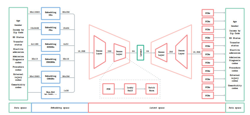
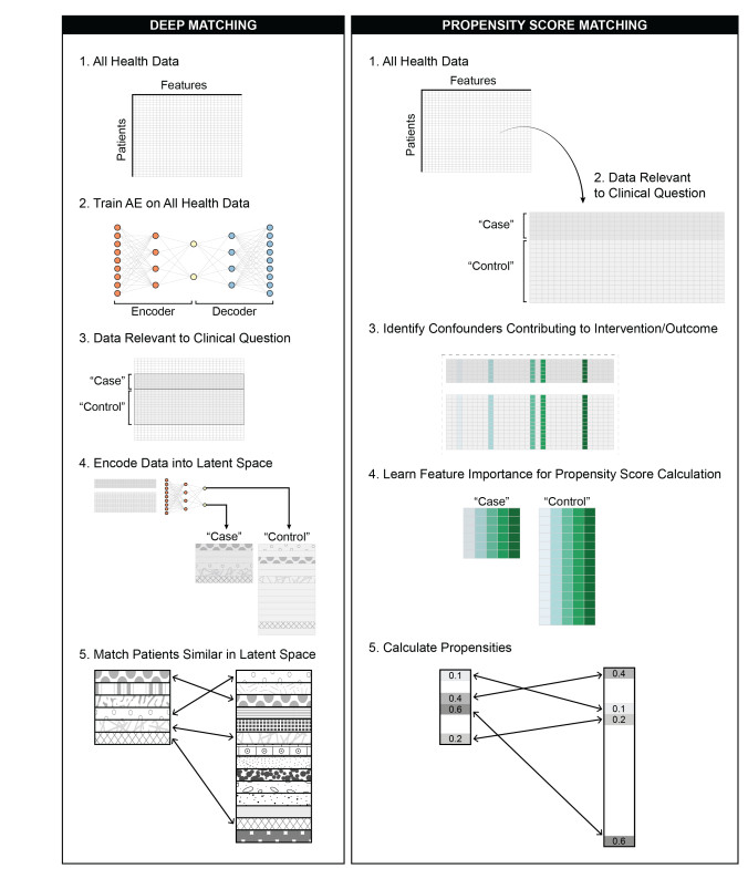
A significant amount of clinical research is observational by nature and derived from medical records, clinical trials, and large-scale registries. While there is no substitute for randomized, controlled experimentation, such experiments or trials are often costly, time consuming, and even ethically or practically impossible to execute. Combining classical regression and structural equation modeling with matching techniques can leverage the value of observational data. Nevertheless, identifying variables of greatest interest in high-dimensional data is frequently challenging, even with application of classical dimensionality reduction and/or propensity scoring techniques. Here, we demonstrate that projecting high-dimensional medical data onto a lower-dimensional manifold using deep autoencoders and post-hoc generation of treatment/control cohorts based on proximity in the lower-dimensional space results in better matching of confounding variables compared to classical propensity score matching (PSM) in the original high-dimensional space ($ P < 0.0001 $) and performs similarly to PSM models constructed by experts with prior knowledge of the underlying pathology when evaluated on predicting risk ratios from real-world clinical data. Thus, in cases when the underlying problem is poorly understood and the data is high-dimensional in nature, matching in the autoencoder latent space might be of particular benefit.
- artificial intelligence,
- autoencoders,
- cohort matching,
- data visualization,
- deep learning,
- manifold learning
Citation: Rachel Gologorsky, Sulaiman S. Somani, Sean N. Neifert, Aly A. Valliani, Katherine E. Link, Viola J. Chen, Anthony B. Costa, Eric K. Oermann. Population scale latent space cohort matching for the improved use and exploration of observational trial data[J]. Mathematical Biosciences and Engineering, 2022, 19(7): 6795-6813. doi: 10.3934/mbe.2022320

Related Papers:

Abstract

A significant amount of clinical research is observational by nature and derived from medical records, clinical trials, and large-scale registries. While there is no substitute for randomized, controlled experimentation, such experiments or trials are often costly, time consuming, and even ethically or practically impossible to execute. Combining classical regression and structural equation modeling with matching techniques can leverage the value of observational data. Nevertheless, identifying variables of greatest interest in high-dimensional data is frequently challenging, even with application of classical dimensionality reduction and/or propensity scoring techniques. Here, we demonstrate that projecting high-dimensional medical data onto a lower-dimensional manifold using deep autoencoders and post-hoc generation of treatment/control cohorts based on proximity in the lower-dimensional space results in better matching of confounding variables compared to classical propensity score matching (PSM) in the original high-dimensional space ($ P < 0.0001 $) and performs similarly to PSM models constructed by experts with prior knowledge of the underlying pathology when evaluated on predicting risk ratios from real-world clinical data. Thus, in cases when the underlying problem is poorly understood and the data is high-dimensional in nature, matching in the autoencoder latent space might be of particular benefit.

References

[1]	H. Sacks, T. C. Chalmers, H. S. Jr, Randomized versus historical controls for clinical trials, Am. J. Med., 72 (1982), 233–240. https://doi.org/10.1016/0002-9343(82)90815-4 doi: 10.1016/0002-9343(82)90815-4
[2]	V. Butsic, D. J. Lewis, V. C. Radeloff, M. Baumann, T. Kuemmerle, Quasi-experimental methods enable stronger inferences from observational data in ecology, Basic Appl. Ecol., 19 (2017), 1–10. https://doi.org/10.1016/j.baae.2017.01.005 doi: 10.1016/j.baae.2017.01.005
[3]	J. Concato, N. Shah, R. I. Horwitz, Randomized, controlled trials, observational studies, and the hierarchy of research designs, N. Engl. J. Med., 342 (2000), 1887–1892. https://doi.org/10.1056/NEJM200006223422507 doi: 10.1056/NEJM200006223422507
[4]	E. A. Stuart, Matching methods for causal inference: A review and a look forward, Stat. Sci., 25 (2010), 1–21. https://doi.org/10.1214/09-STS313 doi: 10.1214/09-STS313
[5]	J. Pearl, The foundations of causal inference, Sociol. Methodol., 40 (2010), 75–149. https://doi.org/10.1111/j.1467-9531.2010.01228.x doi: 10.1111/j.1467-9531.2010.01228.x
[6]	A. Abadie, G. W. Imbens, Large sample properties of matching estimators for average treatment effects, Econometrica, 74 (2006), 235–267. https://doi.org/10.1111/j.1468-0262.2006.00655.x doi: 10.1111/j.1468-0262.2006.00655.x
[7]	G. E. Hinton, R. R. Salakhutdinov, Reducing the dimensionality of data with neural networks, Science, 313 (2006), 504–507. https://doi.org/10.1126/science.1127647 doi: 10.1126/science.1127647
[8]	M. Atzmon, A. Gropp, Y. Lipman, Isometric autoencoders, preprint, arXiv: 2006.09289.
[9]	F. Pedregosa, G. Varoquaux, A. Gramfort, V. Michel, B. Thirion, O. Grisel, et al., Scikit-learn: Machine learning in python, J. Mach. Learn. Res., 12 (2011), 2825–2830. https://doi.org/10.48550/arXiv.1201.0490 doi: 10.48550/arXiv.1201.0490
[10]	N. Kallus, DeepMatch: Balancing deep covariate representations for causal inference using adversarial training, in Proceedings of the 37th International Conference on Machine Learning, 119 (2020), 5067–5077.
[11]	N. Kallus, Optimal a priori balance in the design of controlled experiments, J. R. Stat. Soc., 80 (2018), 85–112. https://doi.org/10.1111/rssb.12240 doi: 10.1111/rssb.12240
[12]	F. D. Johansson, U. Shalit, D. Sontag, Learning representations for counterfactual inference, in Proceedings of the 33rd International Conference on Machine Learning, 48 (2016), 3020–3029.
[13]	A. J. Averitt, N. Vanitchanant, R. Ranganath, A. J. Perotte, The counterfactual $\chi$-GAN: Finding comparable cohorts in observational health data, J. Biomed. Inform., 109 (2020), 103515. https://doi.org/10.1016/j.jbi.2020.103515 doi: 10.1016/j.jbi.2020.103515
[14]	G. Alain, Y. Bengio, What regularized Auto-Encoders learn from the Data-Generating distribution, J. Mach. Learn. Res., 2012. https://doi.org/10.48550/arXiv.1211.4246
[15]	Scikit-learn, scikit-learn/scikit-learn, https://github.com/scikit-learn/scikit-learn
[16]	Hcup, Agency for healthcare research and quality, healthcare cost and utilization project HCUP-US NIS overview, https://www.hcup-us.ahrq.gov/nisoverview.jsp, 2012.
[17]	Hcup, Agency for healthcare research and quality, healthcare cost and utilization project, NIS database documentation, https://www.hcup-us.ahrq.gov/db/nation/nis/nisdbdocumentation.jsp, 2012.
[18]	S. Vedantham, S. Z. Goldhaber, J. A. Julian, S. R. Kahn, M. R. Jaff, D. J. Cohen, et al., Pharmacomechanical Catheter-Directed thrombolysis for Deep-Vein thrombosis, N. Engl. J. Med., 377 (2017), 2240–2252. https://doi.org/10.1056/NEJMoa1615066 doi: 10.1056/NEJMoa1615066
[19]	M. Alkhouli, C. J. Zack, H. Zhao, I. Shafi, R. Bashir, Comparative outcomes of catheter-directed thrombolysis plus anticoagulation versus anticoagulation alone in the treatment of inferior vena caval thrombosis, Circ. Cardiovasc. Interv., 8 (2015), e001882. https://doi.org/10.1016/j.jvs.2015.07.046 doi: 10.1016/j.jvs.2015.07.046
[20]	H. S. Gurm, J. S. Yadav, P. Fayad, B. T. Katzen, G. J. Mishkel, T. K. Bajwa, et al., Long-term results of carotid stenting versus endarterectomy in high-risk patients, N. Engl. J. Med., 358 (2008), 1572–1579. https://doi.org/10.1056/NEJMoa0708028 doi: 10.1056/NEJMoa0708028
[21]	L. K. Kim, D. C. Yang, R. V. Swaminathan, R. M. Minutello, P. M. Okin, M. K. Lee, et al., Comparison of trends and outcomes of carotid artery stenting and endarterectomy in the united states, 2001 to 2010, Circ. Cardiovasc. Interv., 7 (2014), 692–700. https://doi.org/10.1161/CIRCINTERVENTIONS.113.001338 doi: 10.1161/CIRCINTERVENTIONS.113.001338
[22]	J. L. Mas, G. Chatellier, B. Beyssen, A. Branchereau, T. Moulin, J. P. Becquemin, et al., Endarterectomy versus stenting in patients with symptomatic severe carotid stenosis, N. Engl. J. Med., 355 (2006), 1660–1671. https://doi.org/10.1056/NEJMoa061752 doi: 10.1056/NEJMoa061752
[23]	K. Kimura, K. Minematsu, T. Yamaguchi, Japan Multicenter Stroke Investigators' Collaboration (J-MUSIC), Atrial fibrillation as a predictive factor for severe stroke and early death in 15,831 patients with acute ischaemic stroke, J. Neurol. Neurosurg. Psychiatry, 76 (2005), 679–683. https://doi.org/10.1136/jnnp.2004.048827 doi: 10.1136/jnnp.2004.048827
[24]	K. Keller, L. Hobohm, P. Wenzel, T. Münzel, C. Espinola-Klein, M. A. Ostad, Impact of atrial fibrillation/flutter on the in-hospital mortality of ischemic stroke patients, Heart Rhythm, 17 (2020), 383–390. https://doi.org/10.1016/j.hrthm.2019.10.001 doi: 10.1016/j.hrthm.2019.10.001
[25]	H. S. Jørgensen, H. Nakayama, J. Reith, H. O. Raaschou, T. S. Olsen, Acute stroke with atrial fibrillation. the copenhagen stroke study, Stroke, 27 (1996), 1765–1769. https://doi.org/10.1161/01.STR.27.10.1765 doi: 10.1161/01.STR.27.10.1765
[26]	Spotify, spotify/annoy, https://github.com/spotify/annoy
[27]	CannyLab, CannyLab/tsne-cuda, https://github.com/CannyLab/tsne-cuda
[28]	Rapidsai, rapidsai/cuml, https://github.com/rapidsai/cuml

Reader Comments

Your name:*

Email:*
© 2022 the Author(s), licensee AIMS Press. This is an open access article distributed under the terms of the Creative Commons Attribution License (http://creativecommons.org/licenses/by/4.0)