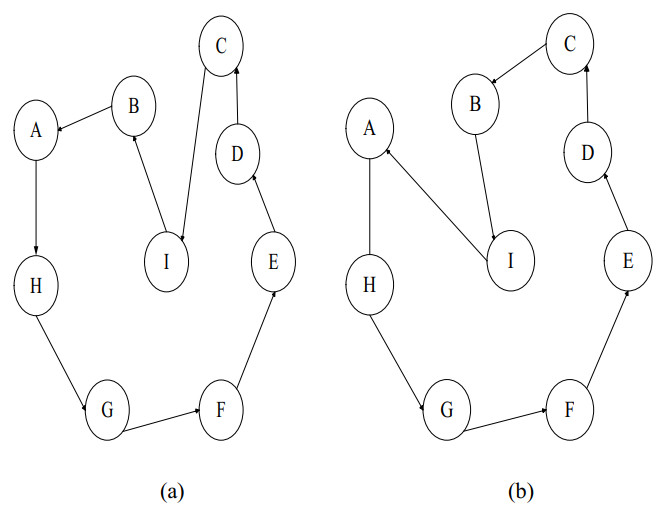
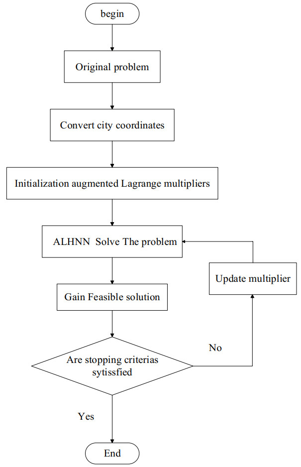
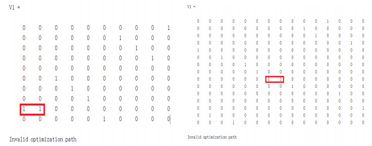
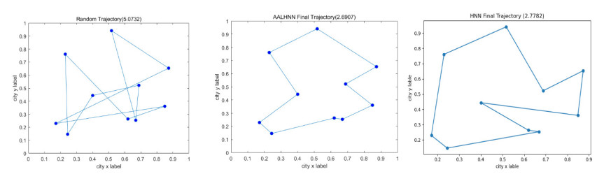
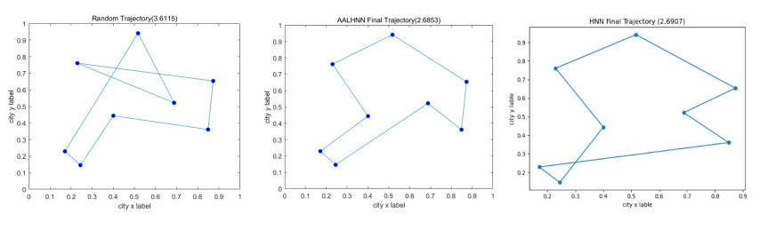
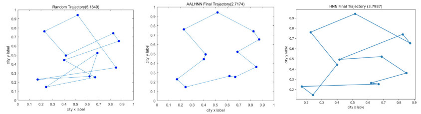
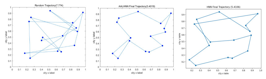
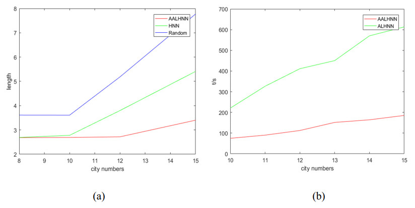
It is prone to get stuck in a local minimum when solving the Traveling Salesman Problem (TSP) by the traditional Hopfield neural network (HNN) and hard to converge to an efficient solution, resulting from the defect of the penalty method used by the HNN. In order to mend this defect, an accelerated augmented Lagrangian Hopfield neural network (AALHNN) algorithm was proposed in this paper. This algorithm gets out of the dilemma of penalty method by Lagrangian multiplier method, ensuring that the solution to the TSP is undoubtedly efficient. The second order factor added in the algorithm stabilizes the neural network dynamic model of the problem, thus improving the efficiency of solution. In this paper, when solving the TSP by AALHNN, some changes were made to the TSP models of Hopfield and Tank. Say, constraints of TSP are multiplied by Lagrange multipliers and augmented Lagrange multipliers respectively, The augmented Lagrange function composed of path length function can ensure robust convergence and escape from the local minimum trap. The Lagrange multipliers are updated by using nesterov acceleration technique. In addition, it was theoretically proved that the extremum obtained by this improved algorithm is the optimal solution of the initial problem and the approximate optimal solution of the TSP was successfully obtained several times in the simulation experiment. Compared with the traditional HNN, this method can ensure that it is effective for TSP solution and the solution to the TSP obtained is better.
Citation: Yun Hu, Qianqian Duan. Solving the TSP by the AALHNN algorithm[J]. Mathematical Biosciences and Engineering, 2022, 19(4): 3427-3448. doi: 10.3934/mbe.2022158
It is prone to get stuck in a local minimum when solving the Traveling Salesman Problem (TSP) by the traditional Hopfield neural network (HNN) and hard to converge to an efficient solution, resulting from the defect of the penalty method used by the HNN. In order to mend this defect, an accelerated augmented Lagrangian Hopfield neural network (AALHNN) algorithm was proposed in this paper. This algorithm gets out of the dilemma of penalty method by Lagrangian multiplier method, ensuring that the solution to the TSP is undoubtedly efficient. The second order factor added in the algorithm stabilizes the neural network dynamic model of the problem, thus improving the efficiency of solution. In this paper, when solving the TSP by AALHNN, some changes were made to the TSP models of Hopfield and Tank. Say, constraints of TSP are multiplied by Lagrange multipliers and augmented Lagrange multipliers respectively, The augmented Lagrange function composed of path length function can ensure robust convergence and escape from the local minimum trap. The Lagrange multipliers are updated by using nesterov acceleration technique. In addition, it was theoretically proved that the extremum obtained by this improved algorithm is the optimal solution of the initial problem and the approximate optimal solution of the TSP was successfully obtained several times in the simulation experiment. Compared with the traditional HNN, this method can ensure that it is effective for TSP solution and the solution to the TSP obtained is better.

| [1] |
J. J. Hopfield, D. W. Tank, "Neural" computation of decisions in optimization problems, Biol. Cybern., 52 (1985), 141–152. https://doi.org/10.1007/BF00339943 doi: 10.1007/BF00339943

|
| [2] |
J. J. Hopfield, Neurons with graded response have collective computational properties like those of two-state neurons, Proc. Natl. Acad. Sci., 81 (1984), 3088–3092. https://doi.org/10.1073/pnas.81.10.3088 doi: 10.1073/pnas.81.10.3088
|
| [3] |
L. Zhang, Y. Zhu, W. X. Zheng, State estimation of discrete-time switched neural networks with multiple communication channels, IEEE Trans. Cybern., 47 (2017), 1028–1040. https://doi.org/10.1109/TCYB.2016.2536748 doi: 10.1109/TCYB.2016.2536748
|
| [4] |
G. V. Wilson, G. S. Pawley, On the stability of the travelling salesman problem algorithm of Hopfield and Tank, Biol. Cybern., 58 (1988), 63–70. https://doi.org/10.1007/BF00363956 doi: 10.1007/BF00363956
|
| [5] | Brandt, W. Yao, Laub, Mitra, Alternative networks for solving the traveling salesman problem and the list-matching problem, in IEEE 1988 International Conference on Neural Networks, (1988), 333–340. https://doi.org/10.1109/ICNN.1988.23945 |
| [6] |
M. Waqas, A. A. Bhatti, Optimization of n + 1 queens problem using discrete neural network, Neural Network World, 27 (2017), 295–308. http://dx.doi.org/10.14311/NNW.2017.27.016 doi: 10.14311/NNW.2017.27.016
|
| [7] | L. García, P. M. Talaván, J. Yáez, The 2-opt behavior of the Hopfield Network applied to the TSP, Oper. Res., 2020. https://doi.org/10.1007/s12351-020-00585-3 |
| [8] |
I. Valova, C. Harris, T. Mai, N. Gueorguieva, Optimization of convolutional neural networks for imbalanced set classification, Procedia Comput. Sci., 176 (2020), 660–669. https://doi.org/10.1016/j.procs.2020.09.038 doi: 10.1016/j.procs.2020.09.038
|
| [9] | S. Z. Li, Relaxation labeling using Lagrange-Hopfield method, in IEEE International Conference on Image Processing, 1 (1995), 266–269. https://doi.org/10.1109/ICIP.1995.529697 |
| [10] | D. Kaznachey, A. Jagota, S. Das, Primal-target neural net heuristics for the hypergraph k-coloring problem, in Proceedings of International Conference on Neural Networks, 2 (1997), 1251–1255. https://doi.org/10.1109/ICNN.1997.616213 |
| [11] |
Z. Wu, Jiang, B. Jiang, H. R. Karimi, A logarithmic descent direction algorithm for the quadratic knapsack problem, Appl. Math. Comput., 369 (2020), 124854. https://doi.org/10.1016/j.amc.2019.124854 doi: 10.1016/j.amc.2019.124854
|
| [12] |
P. V. Yekta, F. J. Honar, M. N. Fesharaki, Modelling of hysteresis loop and magnetic behaviour of fe-48ni alloys using artificial neural network coupled with genetic algorithm, Comput. Mater. Sci., 159 (2019), 349–356. https://doi.org/10.1016/j.commatsci.2018.12.025 doi: 10.1016/j.commatsci.2018.12.025
|
| [13] | A. Rachmad, E. M. S. Rochman, D. Kuswanto, I. Santosa, R. K. Hapsari, T. Indriyani, Comparison of the traveling salesman problem analysis using neural network method, in Proceedings of the International Conference on Science and Technology (ICST), 2018. https://doi.org/10.2991/icst-18.2018.213 |
| [14] | A. Mazeev, A. Semenov, A. Simonov, A distributed parallel algorithm for the minimum spanning tree problem, in International Conference on Parallel Computational Technologies, 753 (2017), 101–113. https://doi.org/10.1007/978-3-319-67035-5_8 |
| [15] |
S. Z. Li, Improving convergence and solution quality of hopfield-type neural networks with augmented lagrange multipliers, IEEE Trans. Neural Networks, 7 (1996). 1507–1516. https://doi.org/10.1109/72.548179 doi: 10.1109/72.548179
|
| [16] |
M. Honari-Latifpour, M. A. Miri, Optical potts machine through networks ofthree-photon down-conversion oscillators, Nanophotonics, 9 (2020), 4199–4205. https://doi.org/10.1515/nanoph-2020-0256 doi: 10.1515/nanoph-2020-0256
|
| [17] |
S. Zhang, A. G. Constantinides, Lagrange programming neural networks, IEEE Trans. Circuits Syst., 39 (1992), 441–452. https://doi.org/10.1109/82.160169 doi: 10.1109/82.160169
|
| [18] | S. S. Kia, An Augmented Lagrangian distributed algorithm for an in-network optimal resource allocation problem, in 2017 American Control Conference (ACC), (2017), 3312–3317. https://doi.org/10.23919/ACC.2017.7963458 |
| [19] |
Y. Hu, Z. Zhang, Y. Yao, X. Huyan, X. Zhou, W. S. Lee, A bidirectional graph neural network for traveling salesman problems on arbitrary symmetric graphs, Eng. Appl. Artif. Intell., 97 (2021), 104061. https://doi.org/10.1016/j.engappai.2020.104061 doi: 10.1016/j.engappai.2020.104061
|
| [20] |
U. Wen, K. M. Lan, H. S. Shih, A review of hopfield neural networks for solving mathematical programming problems, Eur. J. Oper. Res., 198 (2009). 675–687. https://doi.org/10.1016/j.ejor.2008.11.002 doi: 10.1016/j.ejor.2008.11.002
|
| [21] | S. Sangalli, E. Erdil, A. Hoetker, O. Donati, E. Konukoglu, Constrained optimization to train neural networks on critical and under-represented classes, preprient, arXiv: 2102.12894v4. |
| [22] | B. Aylaj, M. Belkasmi, H. Zouaki, A. Berkani, Degeneration simulated annealing algorithm for combinatorial optimization problems, in 2015 15th International Conference on Intelligent Systems Design and Applications (ISDA), (2015), 557–562. https://doi.org/10.1109/ISDA.2015.7489177 |
| [23] |
M. Zarco, T. Froese, Self-modeling in hopfield neural networks with continuous activation function, Procedia Comput. Sci., 123 (2018), 573–578. https://doi.org/10.1016/j.procs.2018.01.087 doi: 10.1016/j.procs.2018.01.087
|
| [24] |
Y. J. Cha, W. Choi, G. Suh, S. Mahmoudkhani, O. Büyüköztürk, Autonomous structural visual inspection using region-based deep learning for detecting multiple damage types, Comput.-Aided Civ. Infrastruct. Eng., 33 (2017), 731–747. https://doi.org/10.1111/mice.12334 doi: 10.1111/mice.12334
|
| [25] | H. Uzawa, K. Arrow, L. Hurwicz, Studies in linear and nonlinear programming, (1958), 154–165. |
| [26] | A. Barra, M. Beccaria, A. Fachechi, A relativistic extension of hopfield neural networks via the mechanical analogy, preprient, arXiv: 1801.01743. |
| [27] |
V. N. Dieu, W. Ongsakul, J. Polprasert, The augmented lagrange hopfield network for economic dispatch with multiple fuel options, Math. Comput. Modell., 57 (2013), 30–39. https://doi.org/10.1016/j.mcm.2011.03.041 doi: 10.1016/j.mcm.2011.03.041
|
| [28] | Y. Arjevani, J. Bruna, B. Can, M. Gürbüzbalaban, S. Jegelka, H. Lin, Ideal: inexact decentralized accelerated augmented lagrangian method, preprient, arXiv: 2006.06733. |
| [29] |
C. Dang, L. Xu, A lagrange multiplier and hopfield-type barrier function method for the traveling salesman problem, Neural Comput., 14 (2002), 303–324. https://doi.org/10.1162/08997660252741130 doi: 10.1162/08997660252741130
|
| [30] |
Z. Wu, Q. Gao, B. Jiang, H. R. Karimi, Solving the production transportation problem via a deterministic annealing neural network method, Appl. Math. Comput., 411 (2021), 126518. https://doi.org/10.1016/j.amc.2021.126518 doi: 10.1016/j.amc.2021.126518
|
| [31] |
M. Kang, S. Yun, H. Woo, M. Kang, Accelerated bregman method for linearly constrained ℓ_1-ℓ_2 minimization, J. Sci. Comput., 56 (2013), 515–534. https://doi.org/10.1007/s10915-013-9686-z doi: 10.1007/s10915-013-9686-z
|
Figures(8) / Tables(3)

Yun Hu, Qianqian Duan. Solving the TSP by the AALHNN algorithm[J]. Mathematical Biosciences and Engineering, 2022, 19(4): 3427-3448. doi: 10.3934/mbe.2022158


 DownLoad: