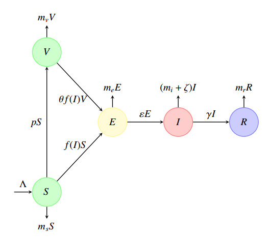
A generalized "SVEIR" epidemic model with general nonlinear incidence rate has been proposed as a candidate model for measles virus dynamics. The basic reproduction number $ \mathcal{R} $, an important epidemiologic index, was calculated using the next generation matrix method. The existence and uniqueness of the steady states, namely, disease-free equilibrium ($ \mathcal{E}_0 $) and endemic equilibrium ($ \mathcal{E}_1 $) was studied. Therefore, the local and global stability analysis are carried out. It is proved that $ \mathcal{E}_0 $ is locally asymptotically stable once $ \mathcal{R} $ is less than. However, if $ \mathcal{R} > 1 $ then $ \mathcal{E}_0 $ is unstable. We proved also that $ \mathcal{E}_1 $ is locally asymptotically stable once $ \mathcal{R} > 1 $. The global stability of both equilibrium $ \mathcal{E}_0 $ and $ \mathcal{E}_1 $ is discussed where we proved that $ \mathcal{E}_0 $ is globally asymptotically stable once $ \mathcal{R}\leq 1 $, and $ \mathcal{E}_1 $ is globally asymptotically stable once $ \mathcal{R} > 1 $. The sensitivity analysis of the basic reproduction number $ \mathcal{R} $ with respect to the model parameters is carried out. In a second step, a vaccination strategy related to this model will be considered to optimise the infected and exposed individuals. We formulated a nonlinear optimal control problem and the existence, uniqueness and the characterisation of the optimal solution was discussed. An algorithm inspired from the Gauss-Seidel method was used to resolve the optimal control problem. Some numerical tests was given confirming the obtained theoretical results.
Citation: Miled El Hajji, Amer Hassan Albargi. A mathematical investigation of an 'SVEIR' epidemic model for the measles transmission[J]. Mathematical Biosciences and Engineering, 2022, 19(3): 2853-2875. doi: 10.3934/mbe.2022131
A generalized "SVEIR" epidemic model with general nonlinear incidence rate has been proposed as a candidate model for measles virus dynamics. The basic reproduction number $ \mathcal{R} $, an important epidemiologic index, was calculated using the next generation matrix method. The existence and uniqueness of the steady states, namely, disease-free equilibrium ($ \mathcal{E}_0 $) and endemic equilibrium ($ \mathcal{E}_1 $) was studied. Therefore, the local and global stability analysis are carried out. It is proved that $ \mathcal{E}_0 $ is locally asymptotically stable once $ \mathcal{R} $ is less than. However, if $ \mathcal{R} > 1 $ then $ \mathcal{E}_0 $ is unstable. We proved also that $ \mathcal{E}_1 $ is locally asymptotically stable once $ \mathcal{R} > 1 $. The global stability of both equilibrium $ \mathcal{E}_0 $ and $ \mathcal{E}_1 $ is discussed where we proved that $ \mathcal{E}_0 $ is globally asymptotically stable once $ \mathcal{R}\leq 1 $, and $ \mathcal{E}_1 $ is globally asymptotically stable once $ \mathcal{R} > 1 $. The sensitivity analysis of the basic reproduction number $ \mathcal{R} $ with respect to the model parameters is carried out. In a second step, a vaccination strategy related to this model will be considered to optimise the infected and exposed individuals. We formulated a nonlinear optimal control problem and the existence, uniqueness and the characterisation of the optimal solution was discussed. An algorithm inspired from the Gauss-Seidel method was used to resolve the optimal control problem. Some numerical tests was given confirming the obtained theoretical results.

| [1] | CDC, Measles (Rubeola), 2020. Available from: https://www.cdc.gov/measles/index.html. |
| [2] |
M. Fakhruddin, D. Suandi, Sumiati, H. Fahlena, N. Nuraini, E. Soewono, Investigation of a measles transmission with vaccination: A case study in Jakarta, Indonesia. Math. Biosci. Eng., 17 (2020), 2998–3018. https://doi.org/10.3934/mbe.2020170. doi: 10.3934/mbe.2020170

|
| [3] | WHO, Measles, 2019. Available from: https://www.who.int/en/news-room/fact-sheets/detail/measles. |
| [4] | O. Diekmann, J. Heesterbeek, Mathematical Epidemiology of Infectious Diseases: Model Building, Analysis, and Interpretation, Jhon Wiley, 2000. |
| [5] |
P. Driessche, J. Watmough, Reproduction numbers and sub-threshold endemic equilibria for compartmental models of disease transmission, Math. Biosci., 180 (2002), 29–48. https://doi.org/10.1016/S0025-5564(02)00108-6. doi: 10.1016/S0025-5564(02)00108-6
|
| [6] |
A. A. Alderremy, J. F. Gómez-Aguilar, S. Aly, K. M. Saad, A fuzzy fractional model of coronavirus (COVID-19) and its study with Legendre spectral method, Results Phys., 21 (2021), 103773. https://doi.org/10.1016/j.rinp.2020.103773. doi: 10.1016/j.rinp.2020.103773
|
| [7] |
D. Aldila, D. Asrianti, A deterministic model of measles with imperfect vaccination and quarantine intervention, J. Phys.: Conf. Ser., 1218 (2019), 012044. https://doi.org/10.1088/1742-6596/1218/1/012044. doi: 10.1088/1742-6596/1218/1/012044
|
| [8] |
M. Sen, S. Alonso-Quesada, Vaccination strategies based on feedback control techniques for a general SEIR-epidemic model, Appl. Math. Comput., 218 (2011), 3888–3904. https://doi.org/10.1016/j.amc.2011.09.036. doi: 10.1016/j.amc.2011.09.036
|
| [9] |
M. El Hajji, S. Sayari, Analysis of a fractional-order "SVEIR" epidemic model with a general nonlinear saturated incidence rate in a continuous reactor, Asian Res. J. Math., 12 (2019), 1–17. https://doi.org/10.9734/arjom/2019/v12i430095. doi: 10.9734/arjom/2019/v12i430095
|
| [10] |
M. El Hajji, Boundedness and asymptotic stability of nonlinear Volterra integro-differential equations using Lyapunov functional, J. King Saud Univ., Sci., 31 (2019), 1516–1521. https://doi.org/10.1016/j.jksus.2018.11.012. doi: 10.1016/j.jksus.2018.11.012
|
| [11] |
M. El Hajji, How can inter-specific interferences explain coexistence or confirm the competitive exclusion principle in a chemostat, Int. J. Biomath., 11 (2018), 1850111. https://doi.org/10.1142/S1793524518501115. doi: 10.1142/S1793524518501115
|
| [12] |
A. B. Gumel, C. C. McCluskey, J. Watmough, An sveir model for assessing potential impact of an imperfect anti-sars vaccine, Math. Biosci. Eng., 3 (2006), 485–512. https://doi.org/10.3934/mbe.2006.3.485. doi: 10.3934/mbe.2006.3.485
|
| [13] | M. El Hajji, N. Chorfi, M. Jleli, Mathematical modelling and analysis for a three-tiered microbial food web in a chemostat, Electron. J. Differ. Equations, 2017 (2017), 1–13. Available from: http://ejde.math.unt.edu. |
| [14] | M. El Hajji, N. Chorfi, M Jleli, Mathematical model for a membrane bioreactor process, Electron. J. Differ. Equations, 2015 (2015), 1–7. Available from: http://ejde.math.txstate.edu. |
| [15] |
M. Farman, A. Ahmad, M. U. Saleem, M. O. Ahmad, Analysis and numerical solution of epidemic models by using nonstandard finite difference scheme, Pure Appl. Biol., 9 (2020), 674–682. http://dx.doi.org/10.19045/bspab.2020.90073. doi: 10.19045/bspab.2020.90073
|
| [16] |
L. Michel, C. J. Silva, D. F. M. Torres, Model-free based control of a HIV/AIDS prevention model, Math. Biosc. Eng., 19 (2022), 759–774. https://doi.org/10.3934/mbe.2022034. doi: 10.3934/mbe.2022034
|
| [17] |
C. J. Silva, G. Cantin, C. Cruz, R. Fonseca-Pinto, R. Passadouro, E. S. dos Santos, et al., Complex network model for COVID-19: Human behavior, pseudo-periodic solutions and multiple epidemic waves, J. Math. Anal. Appli., 2021, 125171. https://doi.org/10.1016/j.jmaa.2021.125171. doi: 10.1016/j.jmaa.2021.125171
|
| [18] |
H. W. Hethcote, The mathematics of infectious diseases, SIAM Rev., 42 (2000), 599–653. https://doi.org/10.1137/S0036144500371907. doi: 10.1137/S0036144500371907
|
| [19] |
I. A. Moneim, An SEIR model with infectious latent and a periodic vaccination strategy, Math. Modell. Anal., 26 (2021), 236–252. https://doi.org/10.3846/mma.2021.12945. doi: 10.3846/mma.2021.12945
|
| [20] |
M. El Hajji, Modelling and optimal control for Chikungunya disease, Theory Biosci., 140 (2021), 27–44. https://doi.org/10.1007/s12064-020-00324-4. doi: 10.1007/s12064-020-00324-4
|
| [21] |
M. El Hajji, S. Sayari, A. Zaghdani, Mathematical analysis of an "SIR" epidemic model in a continuous reactor—deterministic and probabilistic approaches, J. Korean Math. Soc., 58 (2021), 45–67. https://doi.org/10.4134/JKMS.j190788. doi: 10.4134/JKMS.j190788
|
| [22] |
H. W. Hethcote, Three basic epidemiological models, Biomathematics, 18 (1989). https://doi.org/10.1007/978-3-642-61317-3_5. doi: 10.1007/978-3-642-61317-3_5
|
| [23] |
W. O. Kermack, A. G. McKendrick, A contribution to the mathematical theory of epidemics, R. Soc., 115 (1927), 700–721. https://doi.org/10.1098/rspa.1927.0118. doi: 10.1098/rspa.1927.0118
|
| [24] |
S. Edward, E. K. Raymond, T. K. Gabriel, F. Nestory, G. M. Godfrey, P. M. Arbogast, A mathematical model for control and elimination of the transmission dynamics of measles, Appl. Comput. Math., 4 (2015), 396–408. http://doi.org/10.11648/j.acm.20150406.12. doi: 10.11648/j.acm.20150406.12
|
| [25] |
A. A. Momoh, M. O. Ibrahim, I. J. Uwanta, S. B. Manga, Mathematical model for control of measles epidemiology, I. J. Pure Appl. Math., 87 (2013), 707–718. https://doi.org/10.12732/ijpam.v87i5.4. doi: 10.12732/ijpam.v87i5.4
|
| [26] |
H. Wei, Y. Jiang, X. Song, G. H. Su, S. Z. Qiu, Global attractivity and permanence of a SVEIR epidemic model with pulse vaccination and time delay, J. Comput. Appl. Math., 229 (2009), 302–312. https://doi.org/10.1016/j.cam.2008.10.046. doi: 10.1016/j.cam.2008.10.046
|
| [27] | P. Adda, L. N. Nkague, G. Sallet, L. Castelli, A SVEIR model with imperfect vaccine, in CMPD 3 Conference on Computational and Mathematical Population Dynamics, 2010. https://hal.inria.fr/hal-00764764. |
| [28] |
L. N. Nkague, J. M. Ntaganda, H. Abboubakar, J. C. Kamgang, L. Castelli, Global stability of a SVEIR epidemic model: Application to poliomyelitis transmission dynamics, Open J. Modell. Simul., 5 (2017), 98–112. https://doi.org/10.4236/ojmsi.2017.51008. doi: 10.4236/ojmsi.2017.51008
|
| [29] | J. P. LaSalle, The Stability of Dynamical Systems, SIAM, 25 (1976). https://doi.org/10.1137/1.9781611970432. |
| [30] |
M. El Hajji, A. Zaghdani, S. Sayari, Mathematical analysis and optimal control for Chikungunya virus with two routes of infection with nonlinear incidence rate, Int. J. Biomath., (2021), 2150088. https://doi.org/10.1142/S1793524521500881. doi: 10.1142/S1793524521500881
|
| [31] |
N. Chitnis, J. M. Hyman, J. M. Cushing, Determining important parameters in the spread of malaria through the sensitivity analysis of a mathematical model, Bull. Math. Biol., 70 (2008), 1272–1296. https://doi.org/10.1007/s11538-008-9299-0. doi: 10.1007/s11538-008-9299-0
|
| [32] |
C. J. Silva, D. F. M. Torres, Optimal control for a tuberculosis model with reinfection and post-exposure interventions, Math. Biosci., 244 (2013), 154–164. https://doi.org/10.1016/j.mbs.2013.05.005. doi: 10.1016/j.mbs.2013.05.005
|
| [33] |
H. S. Rodrigues, M. T. T. Monteiro, D. F. M. Torres, Sensitivity analysis in a dengue epidemiological model, Conf. Pap. Sci., 2013. https://doi.org/10.1155/2013/721406. doi: 10.1155/2013/721406
|
| [34] | W. Fleming, R. Rishel, Deterministic and Stochastic Optimal Control, Springer Verlag, New York, 1975. https://doi.org/10.1007/978-1-4612-6380-7. |
| [35] | S. Lenhart, J. T. Workman, Optimal Control Applied to Biological Models, Chapman and Hall, 2007. https://doi.org/10.1201/9781420011418. |
| [36] | L. S. Pontryagin, V. G. Boltyanskii, R. V. Gamkrelidze, E. F. Mishchenko, K. N. Trirogoff, L. W. Neustadt, The Mathematical Theory of Optimal Processes, 2000. https://doi.org/10.1201/9780203749319. |
| [37] |
A. B. Gumel, P. N. Shivakumar, B. M. Sahai, A mathematical model for the dynamics of HIV-1 during the typical course of infection, Nonlinear Anal., Theory Methods Appl., 47 (2001), 1773–1783. https://doi.org/10.1016/S0362-546X(01)00309-1. doi: 10.1016/S0362-546X(01)00309-1
|
Figures(4) / Tables(3)

Miled El Hajji, Amer Hassan Albargi. A mathematical investigation of an "SVEIR" epidemic model for the measles transmission[J]. Mathematical Biosciences and Engineering, 2022, 19(3): 2853-2875. doi: 10.3934/mbe.2022131


 DownLoad: