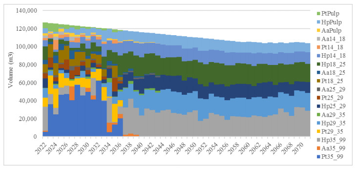
In this paper we evaluate different models and constraints to define strategic planning approaches. In addition, we analyze the best models to meet the expectations generated by the organization. A forest company situated in the province of Misiones, Argentina, provided the data. Hence, forest growth was simulated and, ultimately, optimized planning was used to evaluate different scenarios with 50-year horizon. The best results to stabilize log production were obtained when the harvest is relaxed in ±2 years. Relaxing the clear-cut age leads to a better balance in planting, thinning (1, 2, 3 and 4) and clear felling operations. We found that when maximizing the economic benefit, the NPV is slightly higher, however, this is not significant. In this sense, the planner chooses an economic or volumetric objective function. Furthermore, we demonstrated that model 1 presented better results than model 2 because it manages to stabilize production in the planning horizon. The results allow forest companies to see the implication of choosing the model for strategic planning.
Citation: Diego Broz, Mathías López, Enzo Sanzovo, Julio Arce, Hugo Reis. Evaluation of different strategic planning approaches in a forest plantation in the North of Misiones Province, Argentina[J]. Mathematical Biosciences and Engineering, 2022, 19(1): 918-935. doi: 10.3934/mbe.2022042
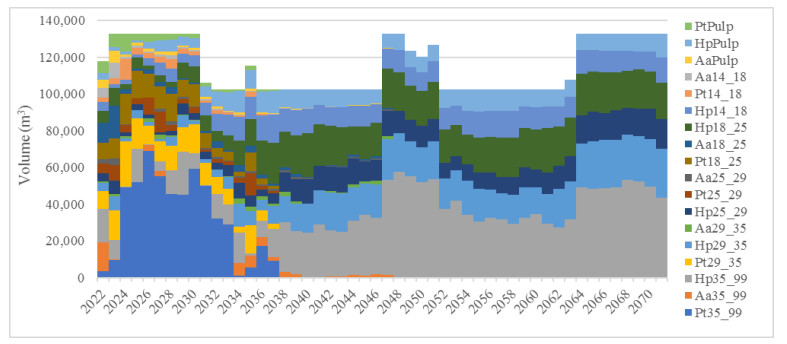
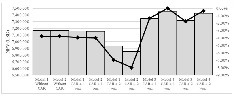
In this paper we evaluate different models and constraints to define strategic planning approaches. In addition, we analyze the best models to meet the expectations generated by the organization. A forest company situated in the province of Misiones, Argentina, provided the data. Hence, forest growth was simulated and, ultimately, optimized planning was used to evaluate different scenarios with 50-year horizon. The best results to stabilize log production were obtained when the harvest is relaxed in ±2 years. Relaxing the clear-cut age leads to a better balance in planting, thinning (1, 2, 3 and 4) and clear felling operations. We found that when maximizing the economic benefit, the NPV is slightly higher, however, this is not significant. In this sense, the planner chooses an economic or volumetric objective function. Furthermore, we demonstrated that model 1 presented better results than model 2 because it manages to stabilize production in the planning horizon. The results allow forest companies to see the implication of choosing the model for strategic planning.

| [1] |
P. Belavenutti, C. Romero, L. Diaz-Balteiro, Integrating strategic and tactical forest-management models within a multicriteria context, Forest Sci., 65 (2019), 178–188. doi: 10.1093/forsci/fxy052. doi: 10.1093/forsci/fxy052

|
| [2] | J. G. Borges, J. Garcia-Gonzalo, S. Marques, V. A. Valdebenito, M. E. McDill, A. O. Falcão, (2014). Strategic management scheduling. In The Management of industrial forest plantations (pp. 171-238). Springer, Dordrecht. doi: 10.1007/978-94-017-8899-1_6. |
| [3] | D. Andersson, Approaches to Integrated Strategic/Tactical Forest Planning. Licentiate thesis. Swedish University of Agricultural Sciences, 2005. |
| [4] |
D. Broz, G. Durand, D. Rossit, F. Tohmé, M. Frutos, Strategic planning in a forest supply chain: a multigoal and multiproduct approach, Can. J. For. Res., 47 (2017), 297–307. doi: 10.1139/cjfr-2016-0299. doi: 10.1139/cjfr-2016-0299
|
| [5] |
D. R. Broz, D. A. Rossit, D. G. Rossit, A. Cavallin, The Argentinian Forest sector: opportunities and challenges in supply chain management, Uncertain Supply Chain Manag., 6 (2018), 375–392. doi: 10.5267/j.uscm.2018.1.001. doi: 10.5267/j.uscm.2018.1.001
|
| [6] |
P. C. Gilmore, R. E. A. Gomory, Linear programming approach to the cutting stock problem, Oper. Res., 9 (1961), 848–859. doi: 10.1287/opre.9.6.849. doi: 10.1287/opre.9.6.849
|
| [7] | F. Curtis, Linear programming the management of a forest property, J. For., 60 (1962), 611–616. |
| [8] | S. Pnevmaticos, S. Mann, Dynamic programming in tree bucking, For. Prod. J., 22 (1972), 26–30. |
| [9] |
K. Johnson, H. Scheurman, Techniques for prescribing optimal timber harvest and in Techniques for prescribing optimal timber harvest and investment under different objectives - Discussion and synthesis, For. Sci., 23 (1977), a0001–z0001. doi: 10.1093/forestscience/23.s1.a0001. doi: 10.1093/forestscience/23.s1.a0001
|
| [10] |
O. Barros, A. Weintraub, Planning for a vertically integrated forest industry, Oper. Res., 30 (1982), 1168–1182. doi: 10.1287/opre.30.6.1168. doi: 10.1287/opre.30.6.1168
|
| [11] |
H. Gassmann, Optimal harvest of a forest in the presence of uncertainty, Can. J. For. Res., 19 (1989), 1267–1274. doi: 10.1139/x89-193. doi: 10.1139/x89-193
|
| [12] |
P. Bellavenutte, W. Chung, L. Diaz-Balteiro, Partitioning and solving large-scale tactical harvest scheduling problems for industrial plantation forests, Can. J. For. Res., 50 (2020), 811–818. doi: 10.1139/cjfr-2019-0425. doi: 10.1139/cjfr-2019-0425
|
| [13] | J. R. Banhara, L. C. E. Rodriguez, F. Seixas, J. M. M. Á. P. Moreira, L. M. S. da Silva, S. R. Nobre, et al., Agendamento otimizado da colheita de madeira de eucaliptos sob restrições operacionais, espaciais e climáticas, Scientia Forestalis, 38 (2010), 85–95. |
| [14] | P. H. Da Silva, Planejamento otimizado da colheita florestal por blocos e talhões integrado à rede de estradas. Tesis de maestría. Universidade Federal do Paraná. Curitiba, Parana, Brasil. 71 pp. 2015. |
| [15] | T. K. Pereira, Planejamento florestal otimizado de plantios de eucalyptus spp. Considerando blocos anuais de colheita. Tesis de grado. Universidade Federal do Paraná. Curitiba, Parana, Brasil. 51 pp. (2016). |
| [16] | V. Viana Céspedes, Optimización en la planificación de servicios de cosecha forestal. Tesis de Maestría. Universidad de la República. 113 pp. (2018). Available from: https://www.colibri.udelar.edu.uy/jspui/bitstream/20.500.12008/18419/1/TM-Cespedes-Viviana.pdf |
| [17] |
G. Paradis, L. LeBel, S. D'Amours, M. Bouchard, On the risk of systematic drift under incoherent hierarchical forest management planning, Can. J. For. Res., 43 (2013), 480–492. doi: 10.1139/cjfr-2012-0334. doi: 10.1139/cjfr-2012-0334
|
| [18] |
J. Troncoso, S. D'Amours, P. Flisberg, M. Rönnqvist, A. Weintraub, A mixed integer programming model to evaluate integrating strategies in the forest value chain—a case study in the Chilean forest industry, Can. J. For. Res., 45 (2015), 937–949. doi: 10.1139/cjfr-2014-0315. doi: 10.1139/cjfr-2014-0315
|
| [19] | M. Silva, A. Weintraub, C. Romero, C. De la Maza, Forest harvesting and environmental protection based on the goal programming approach, For. Sci., 56 (2010), 460–472. |
| [20] |
L. Diaz-Balteiro, J. González-Pachón, C. Romero, Goal programming in forest management: customizing models for the decision-makers preferences, Scand. J. For. Res., 28 (2013), 166–173. doi: 10.1080/02827581.2012.712154. doi: 10.1080/02827581.2012.712154
|
| [21] |
J. C. Giménez, M. Bertomeu, L. Diaz-Balteiro, C. Romero, Optimal harvest scheduling in Eucalyptus plantations under a sustainability perspective, For. Ecol. Manage., 291 (2013), 367–376. doi: 10.1016/j.foreco.2012.11.045. doi: 10.1016/j.foreco.2012.11.045
|
| [22] | P. Bettinger, W. Chung, The key literature of, and trends in, forest-level management planning in North America, 1950-2001, Int. For. Rev., 6 (2004), 40–50. |
| [23] | COIFORM, available from: http://www.coiform.com.ar, (last accessed 2020/8/19). |
| [24] |
P. Bettinger, D. Graetz, J. Sessions, A density-dependent stand-level optimization approach for deriving management prescriptions for interior northwest (USA) landscapes, For. Ecol. Manag., 217 (2005), 171–186. doi: 10.1016/j.foreco.2005.05.060 doi: 10.1016/j.foreco.2005.05.060
|
| [25] |
A. L. D. Augustynczik, J. E. Arce, A. C. L. D. Silva, Planejamento espacial da colheita considerando áreas máximas operacionais, Cerne, 21 (2015), 649–656. doi: 10.1590/01047760201521042006. doi: 10.1590/01047760201521042006
|
| [26] | A. L. D. Augustynczik, Planejamento florestal otimizado considerando áreas mínimas e máximas operacionais de colheita. Master thesis, Universidade Federal do Paraná, 2014. |
| [27] | W. L. Winston, J. B. Goldberg, Operations research: applications and algorithms (Vol. 3). Belmont: Thomson Brooks/Cole, 2004. |
| [28] |
M. E. McDill, An overview of forest management planning and information management, management of industrial forest plantations, (2014), 27–59. doi: 10.1007/978-94-017-8899-1_2. doi: 10.1007/978-94-017-8899-1_2
|
| [29] |
J. P. Vielma, A. T. Murray, D. M. Ryan, A. Weintraub, Improving computational capabilities for addressing volume constraints in forest harvest scheduling problems, Eur. J. Oper.Res., 176 (2007), 1246–1264. doi: 10.1016/j.ejor.2005.09.016. doi: 10.1016/j.ejor.2005.09.016
|
Figures(10) / Tables(6)

Diego Broz, Mathías López, Enzo Sanzovo, Julio Arce, Hugo Reis. Evaluation of different strategic planning approaches in a forest plantation in the North of Misiones Province, Argentina[J]. Mathematical Biosciences and Engineering, 2022, 19(1): 918-935. doi: 10.3934/mbe.2022042


 DownLoad: