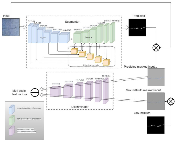
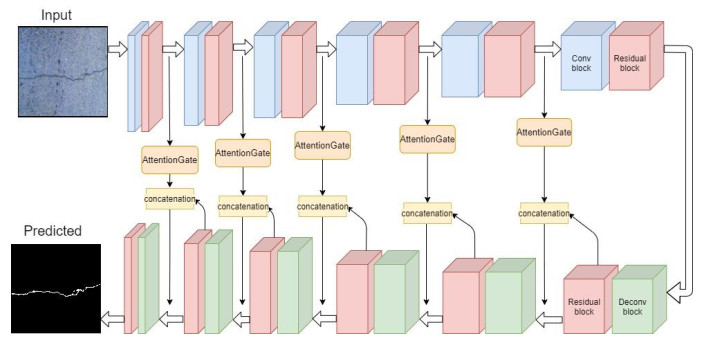
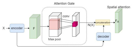
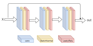
This paper proposed an end-to-end road crack segmentation model based on attention mechanism and deep FCN with generative adversarial learning. We create a segmentation network by introducing a visual attention mechanism and residual module to a fully convolutional network(FCN) to capture richer local features and more global semantic features and get a better segment result. Besides, we use an adversarial network consisting of convolutional layers as a discrimination network. The main contributions of this work are as follows: 1) We introduce a CNN model as a discriminate network to realize adversarial learning to guide the training of the segmentation network, which is trained in a min-max way: the discrimination network is trained by maximizing the loss function, while the segmentation network is trained with the only gradient passed by the discrimination network and aim at minimizing the loss function, and finally an optimal segmentation network is obtained; 2) We add the residual modular and the visual attention mechanism to U-Net, which makes the segmentation results more robust, refined and smooth; 3) Extensive experiments are conducted on three public road crack datasets to evaluate the performance of our proposed model. Qualitative and quantitative comparisons between the proposed method and the state-of-the-art methods show that the proposed method outperforms or is comparable to the state-of-the-art methods in both F1 score and precision. In particular, compared with U-Net, the mIoU of our proposed method is increased about 3%~17% compared with the three public datasets.
Citation: Xing Hu, Minghui Yao, Dawei Zhang. Road crack segmentation using an attention residual U-Net with generative adversarial learning[J]. Mathematical Biosciences and Engineering, 2021, 18(6): 9669-9684. doi: 10.3934/mbe.2021473
This paper proposed an end-to-end road crack segmentation model based on attention mechanism and deep FCN with generative adversarial learning. We create a segmentation network by introducing a visual attention mechanism and residual module to a fully convolutional network(FCN) to capture richer local features and more global semantic features and get a better segment result. Besides, we use an adversarial network consisting of convolutional layers as a discrimination network. The main contributions of this work are as follows: 1) We introduce a CNN model as a discriminate network to realize adversarial learning to guide the training of the segmentation network, which is trained in a min-max way: the discrimination network is trained by maximizing the loss function, while the segmentation network is trained with the only gradient passed by the discrimination network and aim at minimizing the loss function, and finally an optimal segmentation network is obtained; 2) We add the residual modular and the visual attention mechanism to U-Net, which makes the segmentation results more robust, refined and smooth; 3) Extensive experiments are conducted on three public road crack datasets to evaluate the performance of our proposed model. Qualitative and quantitative comparisons between the proposed method and the state-of-the-art methods show that the proposed method outperforms or is comparable to the state-of-the-art methods in both F1 score and precision. In particular, compared with U-Net, the mIoU of our proposed method is increased about 3%~17% compared with the three public datasets.

| [1] | Li. Q, Liu. X, Novel approach to pavement image segmentation based on neighboring difference histogram method, in 2008 Congress on Image and Signal Processing, IEEE, (2008), 792–796. |
| [2] | M. S. Kaseko, S. G. Ritchie, A neural network-based methodology for pavement crack detection and classification, Transport. Res. C.-Emer., 1 (1993), 275–291. |
| [3] | M. Gavilán, D. Balcones, O. Marcos, Adaptive road crack detection system by pavement classification, Sensors, 11 (2011), 9628–9657. |
| [4] | T. S. Nguyen, S. Begot, F. Duculty, Free-form anisotropy: A new method for crack detection on pavement surface images, in 2011 18th IEEE International Conference on Image Processing, IEEE, (2011), 1069–1072. |
| [5] | R. Amhaz, S. Chambon, J. Idier, Automatic crack detection on two-dimensional pavement images: An algorithm based on minimal path selection, IEEE. T. Intell. Transp., 17 (2016), 2718–2729. |
| [6] | M. Avila, S. Begot, F. Duculty, 2D image based road pavement crack detection by calculating minimal paths and dynamic programming, in 2014 IEEE International Conference on Image Processing (ICIP), IEEE, (2014), 783–787. |
| [7] | Q. Li., D. Zhang, Q. Zou, 3D laser imaging and sparse points grouping for pavement crack detection, In: A. Scarpas, N. Kringos, I. Al-Qadi, Loizos A, eds, in 2017 25th European Signal Processing Conference (EUSIPCO), (2017), 2036–2040. |
| [8] | Q. Zou, Y. Cao, Q. Li, CrackTree: Automatic crack detection from pavement images, Pattern. Recogn. Lett., 33 (2012), 227–238. |
| [9] | Y. Huang, Y. J. Tsai, Crack fundamental element (CFE) for multi-scale crack classification, in 7th RILEM International Conference on Cracking in Pavements, (2012), 419–428. |
| [10] | Y. J. Tsai, C. Jiang, Z. Wang, Implementation of automatic crack evaluation using crack fundamental element, in 2014 IEEE International Conference on Image Processing (ICIP), IEEE, (2014), 773–777. |
| [11] | Y. Chen, Y. Zhang, J. Yang, Curve-like structure extraction using minimal path propagation with backtracking, IEEE T. Image. Process, 25 (2015), 988–1003. |
| [12] | K. Y. Song, M. Petrou, J. Kittler, Texture crack detection, Mach. Vision. Appl, 8 (1995): 63–75. |
| [13] | M. Petrou, J. Kittler, K. Y. Song, Automatic surface crack detection on textured materials, J. Mater. Process. Tech., 56 (1996), 158–167. |
| [14] | E. Douka, S. Loutridis, A. Trochidis, Crack identification in plates using wavelet analysis, J. Sound. Vib., 270 (2004), 279–295. |
| [15] | P. Subirats, J. Dumoulin, V. Legeay, Automation of pavement surface crack detection using the continuous wavelet transform, in 2006 International Conference on Image Processing, IEEE, (2006), 3037–3040. |
| [16] | L. Itti, C. Koch, E. Niebur, A model of saliency-based visual attention for rapid scene analysis, IEEE T. Pattern. Anal., 20 (1998), 1254–1259. |
| [17] | W. Xu, Z. Tang, J. Zhou, Pavement crack detection based on saliency and statistical features, in 2013 IEEE International Conference on Image Processing, IEEE, (2013), 4093–4097. |
| [18] | D. Ciresan, A. Giusti, L. Gambardella, Deep neural networks segment neuronal membranes in electron microscopy images, Adv. Neural Inform. Process Syst., 25 (2012), 2843–2851. |
| [19] | Y. J. Cha, W. Choi, O. Büyüköztürk, Deep learning-based crack damage detection using convolutional neural networks, Computer‐Aided Civil Infrast. Eng., 32 (2017), 361–378. |
| [20] | Y. J. Cha, W. Choi, G. Suh, Autonomous structural visual inspection using region-based deep learning for detecting multiple damage types, Computer‐Aided Civil Infrast. Eng., 33 (2018), 731–747. |
| [21] | Y. Liu, J. Yao, X. Lu, DeepCrack: A deep hierarchical feature learning architecture for crack segmentation, Neurocomputing, 338 (2019), 139–153. |
| [22] | J. Long, E. Shelhamer, T. Darrell, Fully convolutional networks for semantic segmentation, in Proceedings of the IEEE conference on computer vision and pattern recognition, IEEE, (2015), 3431–3440. |
| [23] | M. M. Islam, J. M. Kim, Vision-based autonomous crack detection of concrete structures using a fully convolutional encoder–decoder network, Sensors, 19 (2019), 4251. |
| [24] | O. Ronneberger, P. Fischer, T. Brox, U-net: Convolutional networks for biomedical image segmentation, Springer International Publishing, 2015. |
| [25] | O. Oktay, J. Schlemper, L. L. Folgoc, Attention u-net: Learning where to look for the pancreas, 2018. |
| [26] | Z. Liu, Y. Cao, Y. Wang, Computer vision-based concrete crack detection using U-net fully convolutional networks, Automat. Constr., 104 (2019), 129–139. |
| [27] | V. Badrinarayanan, A. Kendall, R. Cipolla, Segnet: A deep convolutional encoder-decoder architecture for image segmentation, IEEE T. Pattern. Anal., 39 (2017), 2481–2495. |
| [28] | Q. Zou, Z. Zhang, Q. Li, Deepcrack: Learning hierarchical convolutional features for crack detection, IEEE T. Image. Process, 28 (2018), 1498–1512. |
| [29] | Y. Liu, J. Yao, X. Lu, DeepCrack: A deep hierarchical feature learning architecture for crack segmentation, Neurocomputing, 338 (2019), 139–153. |
| [30] | F. Wang, M. Jiang, C. Qian, Residual attention network for image classification, in 2017 IEEE Conference on Computer Vision and Pattern Recognition (CVPR), IEEE, (2017), 3156–3164. |
| [31] | D. Yang, H. R. Karimi, K. Sun, Residual wide-kernel deep convolutional auto-encoder for intelligent rotating machinery fault diagnosis with limited samples, Neural Networks, 141 (2021), 133–144. |
| [32] | J. Huyan, W. Li, S. Tighe, CrackU‐net: A novel deep convolutional neural network for pixelwise pavement crack detection, Struct. Contro. Hlth., 27 (2020), e2551. |
| [33] | Z. Fan, C. Li, Y. Chen, Ensemble of deep convolutional neural networks for automatic pavement crack detection and measurement, Coatings, 10 (2020), 152. |
| [34] | W. Song, G. Jia, D. Jia, Automatic pavement crack detection and classification using multiscale feature attention network, IEEE Access, 7 (2019), 171001–171012. |
| [35] | I. Goodfellow, J. Pouget-Abadie, M. Mirza, Generative adversarial networks, Commun. ACM, 63 (2020), 139–144. |
| [36] | P. Luc, C. Couprie, S. Chintala, Semantic segmentation using adversarial networks, in NIPS Workshop on Adversarial Training, 2016. |
| [37] | N. Souly, C. Spampinato, M. Shah, Semi supervised semantic segmentation using generative adversarial network, in Proceedings of the IEEE conference on computer vision and pattern recognition, IEEE, (2017), 5688–5696. |
| [38] | G. Wu, Q. Wang, D. Zhang, A generative probability model of joint label fusion for multi-atlas based brain segmentation, Med. Image. Anal., 18 (2014), 881–890. |
| [39] | V. Alex, M. S. KP, S. S. Chennamsetty, Generative adversarial networks for brain lesion detection, in Medical Imaging 2017: Image Processing-International Society for Optics and Photonics, (2017), 10133: 101330G. |
| [40] | Z. Gao, B. Peng, T. Li, Generative adversarial networks for road crack image segmentation, in 2019 International Joint Conference on Neural Networks (IJCNN), IEEE, (2019), 1–8. |
| [41] | D. Bahdanau, K. Cho, Y. Bengio, Neural machine translation by jointly learning to align and translate, in 3rd International Conference on Learning Representations(ICLR), 2015. |
| [42] | I. J. Goodfellow, J. Shlens, C. Szegedy, Explaining and harnessing adversarial examples, 2014. |
| [43] | A. Madry, A. Makelov, L. Schmidt, Towards deep learning models resistant to adversarial attacks, in International Conference on Learning Representations, 2018. |
| [44] | Y. Shi, L. Cui, Z. Qi, Automatic road crack detection using random structured forests, IEEE T. Intell. Transp., 17 (2016), 3434–3445. |
| [45] | N. T. H. Nguyen, T. H. Le, S. Perry, Pavement crack detection using convolutional neural network, in Proceedings of the Ninth International Symposium on Information and Communication Technology, (2018), 251–256. |
| [46] | M. D. Jenkins, T. A. Carr, M. I. Iglesias, A deep convolutional neural network for semantic pixel-wise segmentation of road and pavement surface cracks, in 2018 26th European Signal Processing Conference (EUSIPCO), IEEE, (2018), 2120–2124. |
| [47] | X. Weng, Y. Huang, W. Wang, Segment-based pavement crack quantification, Automat. Constr., 105 (2019), 102819. |
Figures(8) / Tables(3)

Xing Hu, Minghui Yao, Dawei Zhang. Road crack segmentation using an attention residual U-Net with generative adversarial learning[J]. Mathematical Biosciences and Engineering, 2021, 18(6): 9669-9684. doi: 10.3934/mbe.2021473


 DownLoad: