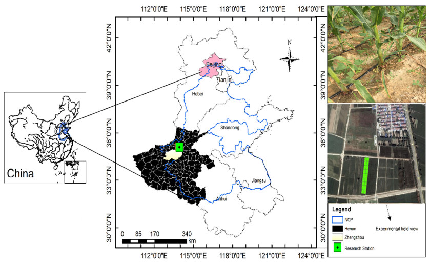
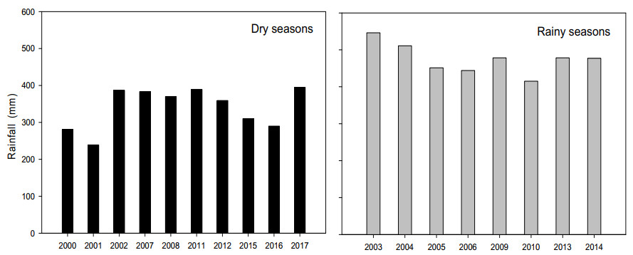
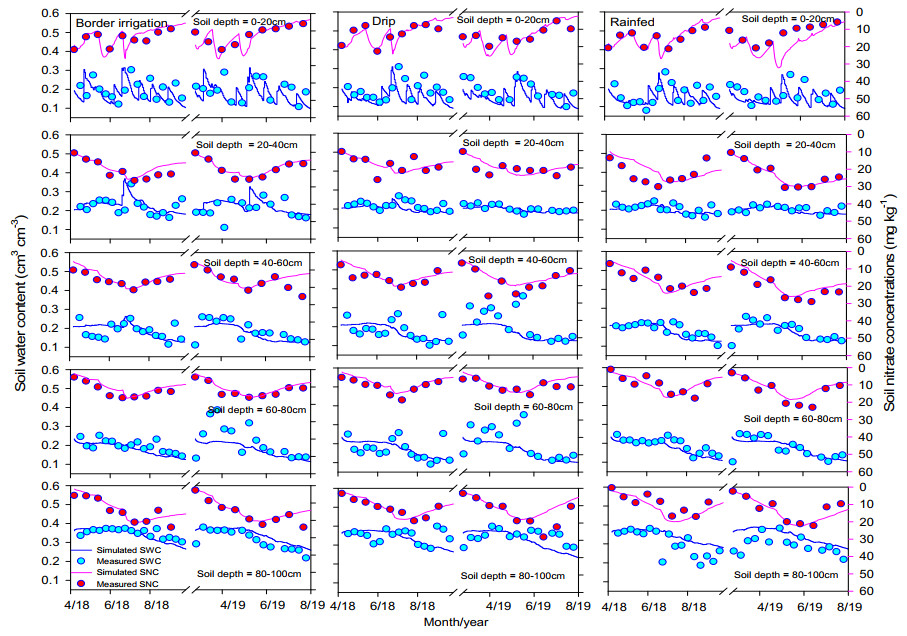
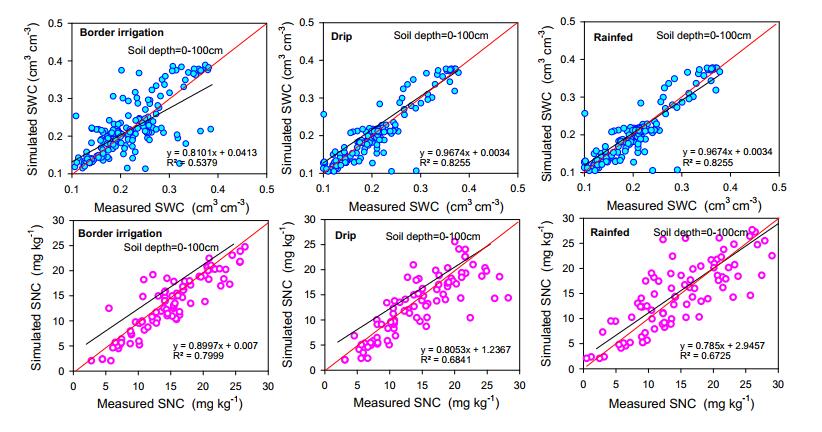
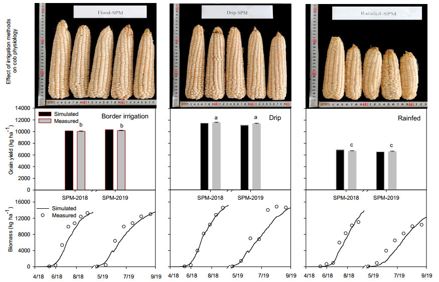
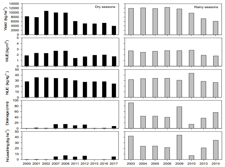
Conventional farming practices not only constrained food security due to low yield but also threatened the ecosystem by causing groundwater decline and groundwater nitrate contamination. A twoear field experiment was conducted at the research station of North China University of Water Resources and Electric Power, Zhengzhou. The WHCNS model was used to simulate grain yield, water and nitrogen fertilizer use efficiencies (WUE and FNUEs) of spring maize under border irrigation method, drip irrigation, and rainfed conditions. In addition, a scenario analysis was also performed on different dry and rainy seasons to assess the long-term impact of rainfall variability on spring maize from 2000–2017. The result showed that the model precisely simulated soil water content, N concentration, crop biomass accumulation, and grain yield. The maximum and minimum range of relative root mean squire error (RRMSE) values were 0.5–36.0% for soil water content, 14.0–38.0% for soil nitrate concentrations, 19.0–24.0% for crop biomass and 1.0–2.0% for grain yield, respectively under three irrigation methods. Both the index of agreement (IA) and Pearson correlation coefficient (r) values were close 1. We found the lowest grain yield from the rainfed maize, whereas the drip irrigation method increased grain yield by 14% at 40% water saving than border irrigation method for the two years with the 11% lower evaporation and maintained transpiration rate. Moreover, the drip irrigated maize had a negligible amount of drainage and runoff, which subsequently improved WUE by 27% in the first growing season and 16% in the second rotation than border irrigation. The drip irrigated maize also showed 24% higher FNUE. The reason of lower WUE and FNUEs under the border irrigation method was increased drainage amounts and N leaching rates. Furthermore, scenario analysis indicated that the dry season could result in a 30.8% yield decline as compared to rainy season.
Citation: Shu Xu, Yichang Wei, Abdul Hafeez Laghari, Xianming Yang, Tongchao Wang. Modelling effect of different irrigation methods on spring maize yield, water and nitrogen use efficiencies in the North China Plain[J]. Mathematical Biosciences and Engineering, 2021, 18(6): 9651-9668. doi: 10.3934/mbe.2021472
Conventional farming practices not only constrained food security due to low yield but also threatened the ecosystem by causing groundwater decline and groundwater nitrate contamination. A twoear field experiment was conducted at the research station of North China University of Water Resources and Electric Power, Zhengzhou. The WHCNS model was used to simulate grain yield, water and nitrogen fertilizer use efficiencies (WUE and FNUEs) of spring maize under border irrigation method, drip irrigation, and rainfed conditions. In addition, a scenario analysis was also performed on different dry and rainy seasons to assess the long-term impact of rainfall variability on spring maize from 2000–2017. The result showed that the model precisely simulated soil water content, N concentration, crop biomass accumulation, and grain yield. The maximum and minimum range of relative root mean squire error (RRMSE) values were 0.5–36.0% for soil water content, 14.0–38.0% for soil nitrate concentrations, 19.0–24.0% for crop biomass and 1.0–2.0% for grain yield, respectively under three irrigation methods. Both the index of agreement (IA) and Pearson correlation coefficient (r) values were close 1. We found the lowest grain yield from the rainfed maize, whereas the drip irrigation method increased grain yield by 14% at 40% water saving than border irrigation method for the two years with the 11% lower evaporation and maintained transpiration rate. Moreover, the drip irrigated maize had a negligible amount of drainage and runoff, which subsequently improved WUE by 27% in the first growing season and 16% in the second rotation than border irrigation. The drip irrigated maize also showed 24% higher FNUE. The reason of lower WUE and FNUEs under the border irrigation method was increased drainage amounts and N leaching rates. Furthermore, scenario analysis indicated that the dry season could result in a 30.8% yield decline as compared to rainy season.

| [1] | Z. Liu, A. Qin, B. Zhao, S. T. Ata-Ul-Karim, J. Xiao, J. Sun, et al., Yield response of spring maize to inter-row subsoiling and soil water deficit in Northern China, PLoS One, 11 (2016). |
| [2] |
W. Feng, M. Zhong, J. M. Lemoine, R. Biancale, H. T. Hsu, J. Xia, Evaluation of groundwater depletion in North China using the Gravity Recovery and Climate Experiment (GRACE) data and ground-based measurements, Water Resour. Res., 49 (2013), 2110–2118. doi: 10.1002/wrcr.20192

|
| [3] |
X. Yang, Y. Chen, S. Pacenka, W. Gao, L. Ma, G. Wang, et al., Effect of diversified crop rotations on groundwater levels and crop water productivity in the North China Plain, J. Hydrol., 522 (2015), 428–438. doi: 10.1016/j.jhydrol.2015.01.010
|
| [4] |
L. Min, Y. Shen, H. Pei, Estimating groundwater recharge using deep vadose zone data under typical irrigated cropland in the piedmont region of the North China Plain, J. Hydrol., 527 (2015), 305–315. doi: 10.1016/j.jhydrol.2015.04.064
|
| [5] | J. Liu, G. Cao, C. Zheng, Sustainability of groundwater resources in the North China Plain, Sustaining Groundwater Res., (2011), 69–87. |
| [6] | X. Yang, Y. Chen, S. Pacenka, W. Gao, M. Zhang, P. Sui, T. S. Steenhuis, Recharge and groundwater use in the north china plain for six irrigated crops for an eleven year period, PLoS One, 10 (2015), 1–17. |
| [7] |
H. Gong, Y. Pan, L. Zheng, X. Li, L. Zhu, C. Zhang, et al., Long-term groundwater storage changes and land subsidence development in the North China Plain (1971–2015), Hydrogeol. J., 26 (2018), 1417–1427. doi: 10.1007/s10040-018-1768-4
|
| [8] | L. Wang, J. Xie, Z. Luo, Y. Niu, J. A. Coulter, R. Zhang, et al., Forage yield, water use efficiency, and soil fertility response to alfalfa growing age in the semiarid Loess Plateau of China, Agric. Water Manage., 243 (2021). |
| [9] | M. N. Khan, M. Mobin, Z. K. Abbas, S. A. Alamri, Fertilizers and their contaminants in soils, surface and groundwater, Encycl. Anthropocene, 5 (2018), 225–240. |
| [10] |
Z. Cui, X. Chen, F. Zhang, Current Nitrogen management status and measures to improve the intensive wheat-maize system in China, Ambio, 39 (2010), 376–384. doi: 10.1007/s13280-010-0076-6
|
| [11] |
J. Letey, P. Vaughan, Soil type, crop and irrigation technique affect nitrogen leaching to groundwater, Calif. Agric., 67 (2013), 231–241. doi: 10.3733/ca.E.v067n04p231
|
| [12] |
X. Ju, C. Zhang, Nitrogen cycling and environmental impacts in upland agricultural soils in North China: A review, J. Integr. Agric., 16 (2017), 2848–2862. doi: 10.1016/S2095-3119(17)61743-X
|
| [13] |
Z. Wang, J. Li, Y. Li, Simulation of nitrate leaching under varying drip system uniformities and precipitation patterns during the growing season of maize in the North China Plain, Agric. Water Manage., 142 (2014), 19–28. doi: 10.1016/j.agwat.2014.04.013
|
| [14] |
Ö. Çetin, E. Akalp, Efficient use of water and fertilizers in irrigated agriculture: drip irrigation and fertigation, Acta Hortic. Regiotect., 22 (2019), 97–102. doi: 10.2478/ahr-2019-0019
|
| [15] |
D. Zaccaria, M. T. Carrillo-Cobo, A. Montazar, D. H. Putnam, K. Bali, Assessing the viability of sub-surface drip irrigation for resource-efficient alfalfa production in central and Southern California, Water, 9 (2017), 837. doi: 10.3390/w9110837
|
| [16] |
M. Umair, T. Hussain, H. Jiang, A. Ahmad, J. Yao, Y. Qi, et al., Water-saving potential of subsurface drip irrigation for winter wheat, Sustainability, 11 (2019), 2978. doi: 10.3390/su11102978
|
| [17] |
H. M. Darouich, C. M. G. Pedras, J. M. Gonçalves, L. S. Pereira, Drip vs. surface irrigation: A comparison focussing on water saving and economic returns using multicriteria analysis applied to cotton, Biosyst. Eng., 122 (2014), 74–90. doi: 10.1016/j.biosystemseng.2014.03.010
|
| [18] | D. Yang, S. Li, S. Kang, T. Du, P. Guo, X. Mao, et al., Effect of drip irrigation on wheat evapotranspiration, soil evaporation and transpiration in Northwest China, Agric. Water Manage., 232 (2020). |
| [19] | Y. Wei, L. Sun, S. Wang, Y. Wang, Z. Zhang, Q. Chen, et al., Effects of different irrigation methods on water distribution and nitrate nitrogen transport of cucumber in greenhouse, Nongye Gongcheng Xuebao/Trans. Chinese Soc. Agric. Eng., 26 (2010), 67–72. |
| [20] |
J. E. Ayars, A. Fulton, B. Taylor, Subsurface drip irrigation in California–Here to stay?, Agric. Water Manage., 157 (2015), 39–47. doi: 10.1016/j.agwat.2015.01.001
|
| [21] |
S. J. Leghari, K. Hu, Y. Wei, T. C. Wang, T. A. Bhutto, M. Buriro, Modelling water consumption, N fates and maize yield under different water-saving management practices in China and Pakistan. Agric. Water Manage., 255 (2021), 107033. doi: 10.1016/j.agwat.2021.107033
|
| [22] | Y. Wang, S. Li, H. Liang, K. Hu, S. Qin, H. Guo, Comparison of water-and nitrogen-use efficiency over drip irrigation with border irrigation based on a model approach, Agronomy, 10 (2020), 1890. |
| [23] |
Z. Zhao, X. Qin, Z. Wang, E. Wang, Performance of different cropping systems across precipitation gradient in North China Plain, Agric. For. Meteorol., 259 (2018), 162–172. doi: 10.1016/j.agrformet.2018.04.019
|
| [24] |
X. L. Yang, Y. Q. Chen, T. S. Steenhuis, S. Pacenka, W. S. Gao, L. Ma, et al., Mitigating groundwater depletion in North China plain with cropping system that alternate deep and shallow rooted crops, Front. Plant Sci., 8 (2017), 980. doi: 10.3389/fpls.2017.00980
|
| [25] | S. Lorvanleuang, Y. Zhao, Automatic irrigation system using android, OALib, 5 (2018). |
| [26] |
J. Wang, P. Wang, Q. Qin, H. Wang, The effects of land subsidence and rehabilitation on soil hydraulic properties in a mining area in the Loess Plateau of China, Catena, 159 (2017), 51–59. doi: 10.1016/j.catena.2017.08.001
|
| [27] | A. N. Beretta, A. V. Silbermann, L. Paladino, D. Torres, D. Bassahun, R. Musselli, et al., Soil texture analyses using a hydrometer: modification of the Bouyoucos method, Cienc. Invest. Agrar., 41 (2014), 263–271. |
| [28] |
M. T. van Genuchten, A closed-form equation for predicting the hydraulic conductivity of unsaturated soils, Soil Sci. Soc. Am. J., 44 (1980), 892–898. doi: 10.2136/sssaj1980.03615995004400050002x
|
| [29] |
S. Zhang, Y. Wei, M. N. Kandhro, F. Wu, Evaluation of FDR MI2X and new WiTu technology sensors to determine soil water content in the corn and weed field, AIMS Agric. Food, 5 (2020), 169–180. doi: 10.3934/agrfood.2020.1.169
|
| [30] |
S. J. Leghari, K. Hu, H. Liang, Y. Wei, Modeling water and nitrogen balance of different cropping systems in the North China Plain, Agronomy, 9 (2019), 696. doi: 10.3390/agronomy9110696
|
| [31] | J. Šimůnek, A. M. Šejna, H. Saito, M. Sakai, M. T. V. Genuchten, The HYDRUS-1D software package for simulating the movement of water, heat, and multiple solutes in variably saturated media, Software Ser., 2013. |
| [32] |
J. D. Hanson, L. R. Ahuja, M. D. Shaffer, K. W. Rojas, D. G. DeCoursey, H. Farahani, et al., RZWQM: Simulating the effects of management on water quality and crop production, Agric. Syst., 57 (1998), 161–195. doi: 10.1016/S0308-521X(98)00002-X
|
| [33] | R. G. Allen, L. S. Pereira, D. Raes, M. Smith, Crop evapotranspiration: Guidelines for computing crop requirements, Irrig. Drain. Pap., 56 (1980) |
| [34] | A. Y. Hachum, J. F. Alfaro, Rain infiltration into layered soils: prediction, J. Irrig. Drain. Div. ASCE., 106 (1980). |
| [35] |
Y. Pachepsky, D. Timlin, W. Rawls, Generalized Richards' equation to simulate water transport in unsaturated soils, J. Hydrol., 272 (2003), 3–13. doi: 10.1016/S0022-1694(02)00251-2
|
| [36] |
J. W. Jung, K. S. Yoon, D. H. Choi, S. S. Lim, W. J. Choi, S. M. Choi, et al., Water management practices and SCS curve numbers of paddy fields equipped with surface drainage pipes, Agric. Water Manage., 110 (2012), 78–83. doi: 10.1016/j.agwat.2012.03.014
|
| [37] | S. Hansen, P. Abrahamsen, C. T. Petersen, M. Styczen, Daisy: model use, calibration, and validation, 55 (2012), 1315–1333. |
| [38] | H. Liang, K. Hu, W. D. Batchelor, Z. Qi, B. Li, An integrated soil-crop system model for water and nitrogen management in North China, Sci. Rep., 6 (2016). |
| [39] |
D. N. Moriasi, J. G. Arnold, M. W. V. Liew, R. L. Bingner, R. D. Harmel, T. L. Veith, Model evaluation guidelines for systematic quantification of accuracy in watershed simulations. Trans., Asabe., 50 (2007), 885–900. doi: 10.13031/2013.23153
|
| [40] |
C. J. Willmott, On the validation of models, Phys. Geogr., 2 (1981), 184–194. doi: 10.1080/02723646.1981.10642213
|
| [41] | M. M. Mukaka, Statistics corner: A guide to appropriate use of correlation coefficient in medical research, Malawi Med. J., 24 (2012), 69–71. |
| [42] | M. Razaq, P. Zhang, H. L. Shen, Salahuddin, Influence of nitrogen and phosphorous on the growth and root morphology of Acer mono, PLoS One, 12 (2017). |
| [43] |
A. A. Siyal, A. S. Mashori, K. L. Bristow, M. T. V. Genuchten, Alternate furrow irrigation can radically improve water productivity of okra, Agric. Water Manage., 173 (2016), 55–60. doi: 10.1016/j.agwat.2016.04.026
|
| [44] | G. Murray-Tortarolo, V. J. Jaramillo, M. Maass, P. Friedlingstein, S. Sitch, The decreasing range between dry- and wet-season precipitation over land and its effect on vegetation primary productivity, PLoS One, 12 (2017). |
| [45] |
X. Gao, X. Chen, T. W. Biggs, H. Yao, Separating wet and dry years to improve calibration of SWAT in Barrett watershed, Southern California, Water, 10 (2018), 274. doi: 10.3390/w10030274
|
| [46] | X. Shi, W. D. Batchelor, H. Liang, S. Li, B. Li, K. Hu, Determining optimal water and nitrogen management under different initial soil mineral nitrogen levels in northwest China based on a model approach, Agric. Water Manage., 234 (2020). |
| [47] |
Y. He, H. Liang, K. Hu, H. Wang, L. Hou, Modeling nitrogen leaching in a spring maize system under changing climate and genotype scenarios in arid Inner Mongolia, China, Agric. Water Manage., 210 (2018), 316–323. doi: 10.1016/j.agwat.2018.08.017
|
| [48] |
H. Liang, K. Hu, W. Qin, Q. Zuo, L. Guo, Y. Tao, et al., Ground cover rice production system reduces water consumption and nitrogen loss and increases water and nitrogen use efficiencies, F. Crop. Res., 233 (2019), 70–79. doi: 10.1016/j.fcr.2019.01.003
|
| [49] | Q. Xu, K. Hu, H. Liang, S. J. Leghari, M. T. Knudsen, Incorporating the WHCNS model to assess water and nitrogen footprint of alternative cropping systems for grain production in the North China Plain, J. Clean. Prod., 263 (2020). |
| [50] |
Y. Liang, Y. Jiang, M. Du, B. Li, L. Chen, M. Chen, et al., ZmASR3 from the maize ASR gene family positively regulates drought tolerance in transgenic arabidopsis, Int. J. Mol. Sci., 20 (2019), 2278. doi: 10.3390/ijms20092278
|
| [51] |
H. Liang, K. Hu, W. Qin, Q. Zuo, Y. Zhang, Modelling the effect of mulching on soil heat transfer, water movement and crop growth for ground cover rice production system, F. Crop. Res., 201 (2017), 97–107. doi: 10.1016/j.fcr.2016.11.003
|
| [52] |
S. K. Jha, T. S. Ramatshaba, G. Wang, Y. Liang, H. Liu, Y. Gao, et al., Response of growth, yield and water use efficiency of winter wheat to different irrigation methods and scheduling in North China Plain, Agric. Water Manage., 217 (2019), 292–302. doi: 10.1016/j.agwat.2019.03.011
|
| [53] | S. Kang, L. Zhang, Y. Liang, X. Hu, H. Cai, B. Gu, Effects of limited irrigation on yield and water use efficiency of winter wheat in the Loess Plateau of China, Agric. Water Manage., 55 (2002), 203–216. |
| [54] |
G. Wang, Q. Fang, B. Wu, H. Yang, Z. Xu, Relationship between soil erodibility and modeled infiltration rate in different soils, J. Hydrol., 528 (2015), 408–418. doi: 10.1016/j.jhydrol.2015.06.044
|
| [55] |
B. Zhou, X. Sun, Z. Ding, W. Ma, M. Zhao, Multisplit nitrogen application via drip irrigation improves maize grain yield and nitrogen use efficiency, Crop Sci., 57 (2017), 1687–1703. doi: 10.2135/cropsci2016.07.0623
|
| [56] |
S. E. El-Hendawy, E. M. Hokam, U. Schmidhalter, Drip irrigation frequency: The effects and their interaction with nitrogen fertilization on sandy soil water distribution, maize yield and water use efficiency under Egyptian conditions, J. Agron. Crop Sci., 194 (2008), 180–192. doi: 10.1111/j.1439-037X.2008.00304.x
|
| [57] |
O. S. Sandhu, R. K. Gupta, H. S. Thind, M. L. Jat, H. S. Sidhu, Yadvinder-Singh, Drip irrigation and nitrogen management for improving crop yields, nitrogen use efficiency and water productivity of maize-wheat system on permanent beds in north-west India, Agric. Water Manage., 219 (2019), 19–26. doi: 10.1016/j.agwat.2019.03.040
|
| [58] | S. J. Leghari, N. A. Wahocho, G. M. Laghari, A. HafeezLaghari, G. MustafaBhabhan, K. H. Talpur, et al., Role of nitrogen for plant growth and development : A review, Adv. Environ. Biol., 10 (2016), 209–218. |
| [59] |
Y. Li, H. Liu, G. Huang, R. Zhang, H. Yang, Nitrate nitrogen accumulation and leaching pattern at a winter wheat: summer maize cropping field in the North China Plain, Environ. Earth Sci., 75 (2016), 118. doi: 10.1007/s12665-015-4867-8
|
| [60] |
D. Wu, X. Xu, Y. Chen, H. Shao, E. Sokolowski, G. Mi, Effect of different drip fertigation methods on maize yield, nutrient and water productivity in two-soils in Northeast China, Agric. Water Manage., 213 (2019), 200–211. doi: 10.1016/j.agwat.2018.10.018
|
| [61] |
A. Gadédjisso-Tossou, T. Avellán, N. Schütze, Potential of deficit and supplemental irrigation under climate variability in northern Togo, West Africa, Water, 10 (2018), 1803.. doi: 10.3390/w10121803
|
| [62] |
W. Zhao, L. Liu, Q. Shen, J. Yang, X. Han, F. Tian, et al., Effects of Water Stress on Photosynthesis, Yield, and Water Use Efficiency in Winter Wheat, Water, 12 (2020), 2127. doi: 10.3390/w12082127
|
| [63] |
Y. Liu, H. Yang, J. Li, Y. Li, H. Yan, Estimation of irrigation requirements for drip-irrigated maize in a sub-humid climate, J. Integr. Agric., 17 (2018), 677–692. doi: 10.1016/S2095-3119(17)61833-1
|
Figures(6) / Tables(5)

Shu Xu, Yichang Wei, Abdul Hafeez Laghari, Xianming Yang, Tongchao Wang. Modelling effect of different irrigation methods on spring maize yield, water and nitrogen use efficiencies in the North China Plain[J]. Mathematical Biosciences and Engineering, 2021, 18(6): 9651-9668. doi: 10.3934/mbe.2021472


 DownLoad: