New insights on novel coronavirus 2019-nCoV/SARS-CoV-2 modelling in the aspect of fractional derivatives and fixed points

Sumati Kumari Panda; Abdon Atangana; Juan J. Nieto; Sumati Kumari Panda; Abdon Atangana; Juan J. Nieto

doi:10.3934/mbe.2021430

Mathematical Biosciences and Engineering

2021, Volume 18, Issue 6: 8683-8726. doi: 10.3934/mbe.2021430

Previous Article Next Article

Research article Special Issues

New insights on novel coronavirus 2019-nCoV/SARS-CoV-2 modelling in the aspect of fractional derivatives and fixed points

1.
Department of Mathematics, GMR Institute of Technology, Rajam-532127, Andhra Pradesh, India
2.
Institute for Groundwater Studies, University of the Free State, Bloemfontein 9300, South Africa
3.
Department of Medical Research, China Medical University Hospital, Taichung, Taiwan
4.
Institute of Mathematics, University of Santiago de Compostela, Santiago de Compostela 15782, Spain
Correction on: Mathematical Biosciences and Engineering 19: 1588-1590

Received: 19 August 2021 Accepted: 16 September 2021 Published: 12 October 2021

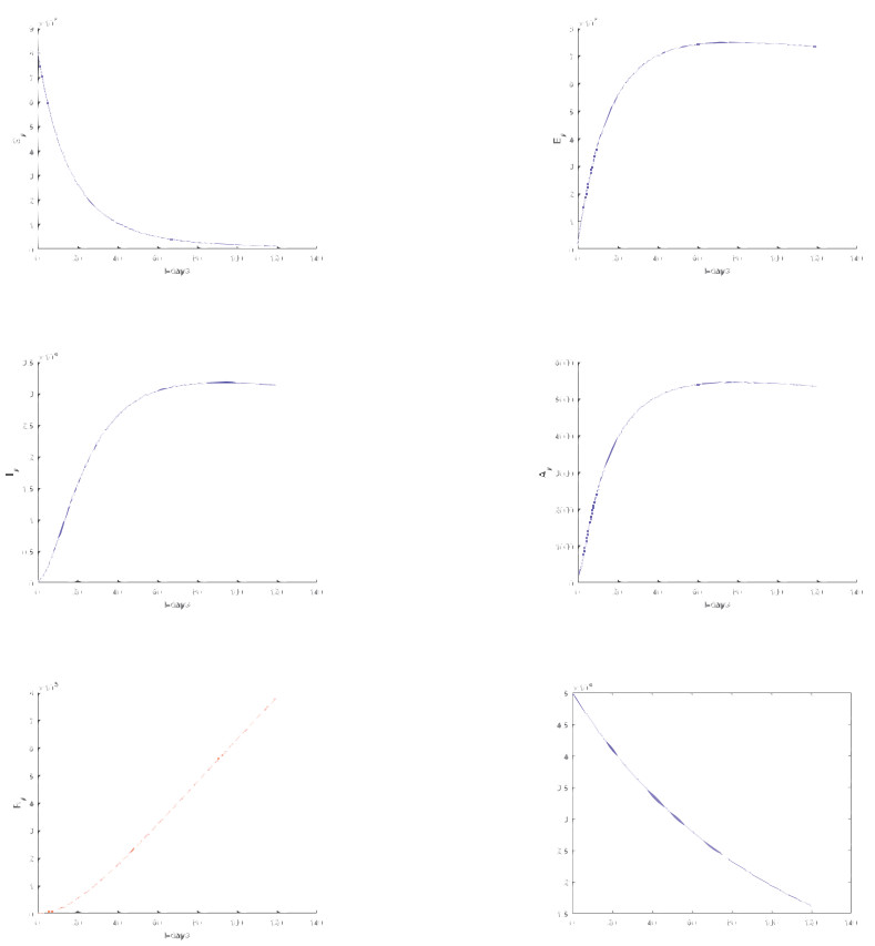
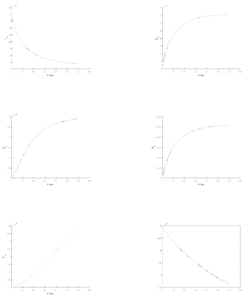
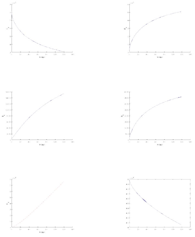
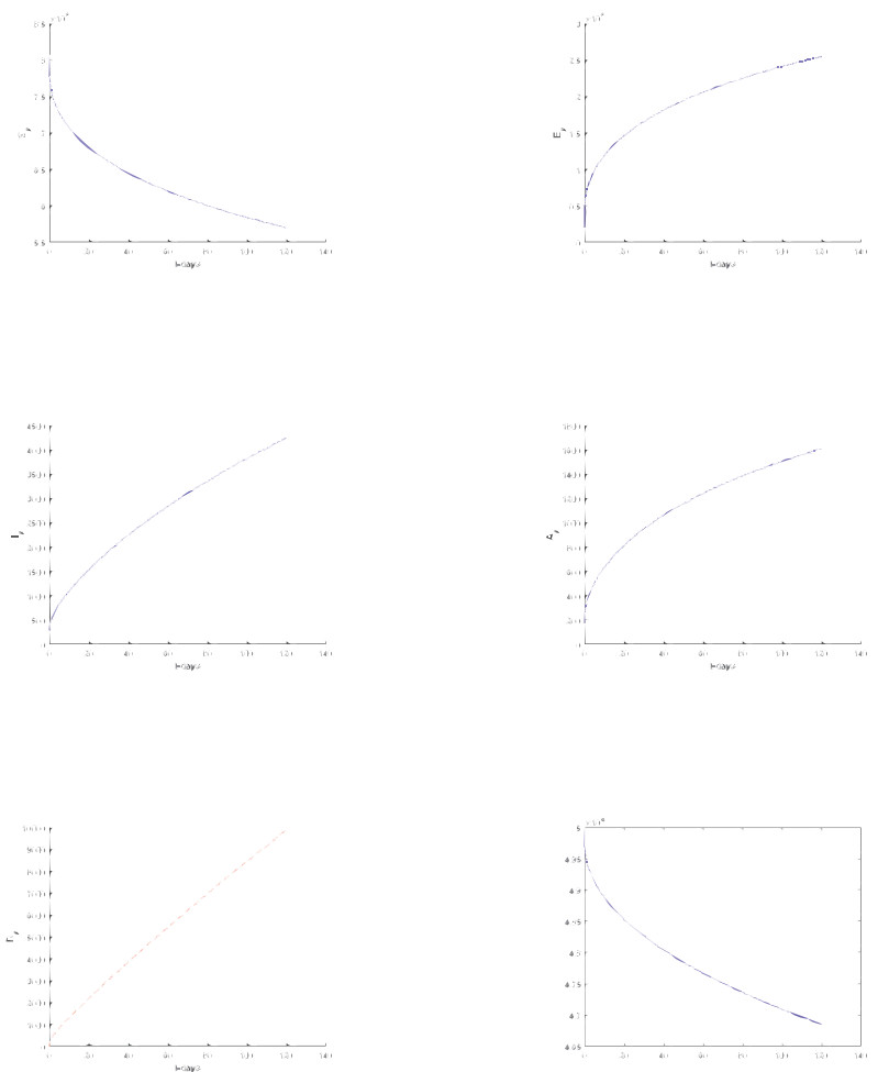
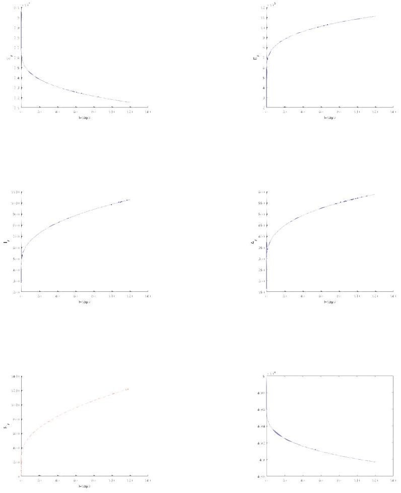
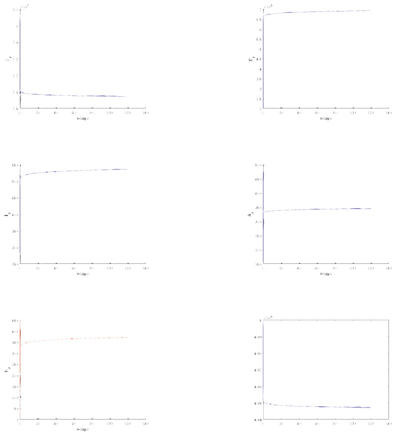
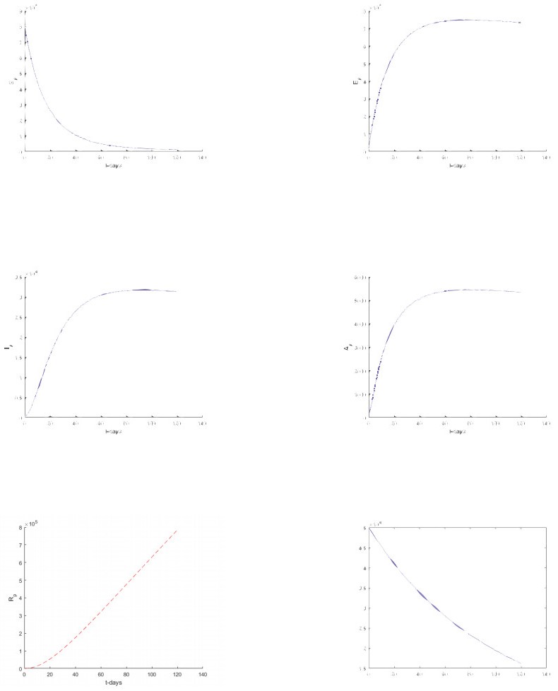
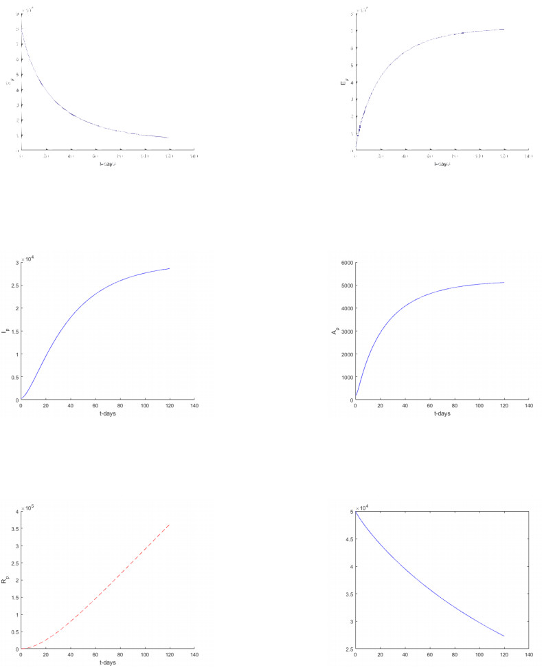
Extended orthogonal spaces are introduced and proved pertinent fixed point results. Thereafter, we present an analysis of the existence and unique solutions of the novel coronavirus 2019-nCoV/SARS-CoV-2 model via fractional derivatives. To strengthen our paper, we apply an efficient numerical scheme to solve the coronavirus 2019-nCoV/SARS-CoV-2 model with different types of differential operators.
Citation: Sumati Kumari Panda, Abdon Atangana, Juan J. Nieto. New insights on novel coronavirus 2019-nCoV/SARS-CoV-2 modelling in the aspect of fractional derivatives and fixed points[J]. Mathematical Biosciences and Engineering, 2021, 18(6): 8683-8726. doi: 10.3934/mbe.2021430

Related Papers:

Abstract

Extended orthogonal spaces are introduced and proved pertinent fixed point results. Thereafter, we present an analysis of the existence and unique solutions of the novel coronavirus 2019-nCoV/SARS-CoV-2 model via fractional derivatives. To strengthen our paper, we apply an efficient numerical scheme to solve the coronavirus 2019-nCoV/SARS-CoV-2 model with different types of differential operators.

References

[1]	Coronavirus disease (COVID-19) pandemic. Available from: https://www.who.int/emergencies/diseases/novel-coronavirus-2019.
[2]	S. Riddell, S. Goldie, A. Hill, D. Eagles, T. W. Drew, The effect of temperature on persistence of SARS-CoV-2 on common surfaces, Virology J., 17 (2020).
[3]	N. van Doremalen, D. H. Morris, M. G. Holbrook, A. Gamble, B. N. Williamson, A. Tamin, et al., Aerosol and surface stability of SARS-CoV-2 as compared with SARS-CoV-1, New Engl. J. Med., 382 (2020), 1564–1567. doi: 10.1056/NEJMc2004973
[4]	S. B. Kasloff, A. Leung, J. E. Strong, D. Funk, T. Cutts, Stability of SARS-CoV-2 on critical personal protective equipment, Sci. Rep., 11 (2021).
[5]	M. A. Khan, A. Atangana, Modeling the dynamics of novel coronavirus (2019-nCov) with fractional derivative, Alexandria Eng. J., 59 (2020), 2379–2389. doi: 10.1016/j.aej.2020.02.033
[6]	A. Atangana, D. Baleanu, New fractional derivatives with nonlocal and non-singular kernel: theory and application to heat transfer model, Therm. Sci., 20 (2016), 763-769. doi: 10.2298/TSCI160111018A
[7]	M. Caputo, M. Fabrizio, A new definition of fractional derivative without singular kernel, Prog. Fract. Differ. Appl., 1 (2015), 1–13.
[8]	J. Losada, J. J. Nieto, Properties of a new fractional derivative without singular kernel, Prog. Fract. Differ. Appl., 1 (2015), 87–92.
[9]	D. Kumar, F. Tchier, J. Singh, D. Baleanu, An efficient computational technique for fractal vehicular traffic flow, Entropy, 20 (2018), 259. doi: 10.3390/e20040259
[10]	E. F. D. Goufo, S. Kumar, S. B. Mugisha, Similarities in a fifth-order evolution equation with and with no singular kernel Chaos Solit. Fract., 130 (2020), 109467.
[11]	A. Atangana, S. I. Araz, RETRACTED: New numerical method for ordinary differential equations: Newton polynomial, J. Comput. Appl. Math., 372 (2020), 112622. doi: 10.1016/j.cam.2019.112622
[12]	A. A. Kilbas, H. M. Srivastava, J. J. Trujillo, Theory and Applications of Fractional Differential Equations, Elsevier Science B.V., Amsterdam, 2006.
[13]	C. Ravichandran, K. Logeswari, F. Jarad, New results on existence in the framework of Atangana-Baleanu derivative for fractional integro-differential equations, Chaos, Solitons Fractals, 125 (2019), 194–200. doi: 10.1016/j.chaos.2019.05.014
[14]	K. Logeswari, C. Ravichandran, A new exploration on existence of fractional neutral integro-differential equations in the concept of Atangana-Baleanu derivative, Phys. A: Stat. Mech. Appl., 544 (2020), 123454. doi: 10.1016/j.physa.2019.123454
[15]	M. A. Alqudah, C. Ravichandran, T. Abdeljawad, N. Valliammal, New results on Caputo fractional-order neutral differential inclusions without compactness, Adv. Differ. Equations, 2019 (2019).
[16]	R. Subashini, K. Jothimani, K. S. Nisar, C. Ravichandran, New results on nonlocal functional integro-differential equations via Hilfer fractional derivative, Alexandria Eng. J., 59 (2019), 2891–2899.
[17]	C. Ravichandran, K. Logeswari, S. K. Panda, K. S. Nisar, On new approach of fractional derivative by Mittag-Leffler kernel to neutral integro-differential systems with impulsive conditions, Chaos, Solitons Fractals, 139 (2020), 110012. doi: 10.1016/j.chaos.2020.110012
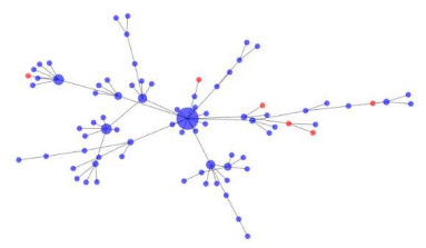
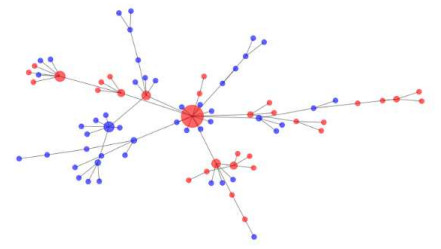
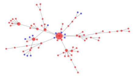
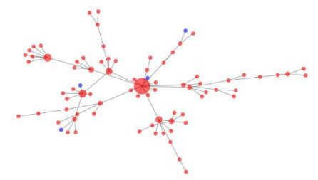
[18]	N. Valliammal, C. Ravichandran, K. S. Nisar, Solutions to fractional neutral delay differential nonlocal systems, Chaos, Solitons Fractals, 138 (2020), 109912. doi: 10.1016/j.chaos.2020.109912
[19]	D. Chalishajar, C. Ravichandran, S. Dhanalakshmi, R. Murugesu, Existence of fractional impulsive functional integro-differential equations in Banach spaces, Appl. Syst. Innovation, 2 (2019), 18. doi: 10.3390/asi2020018
[20]	S. K. Panda, Applying fixed point methods and fractional operators in the modelling of novel coronavirus 2019-nCoV/SARS-CoV-2, Results in Physics, 19 (2020), 103433. doi: 10.1016/j.rinp.2020.103433
[21]	A. Din, Y. Li, Stationary distribution extinction and optimal control for the stochastic hepatitis B epidemic model with partial immunity, Phys. Scr., 96 (2021), 074005. doi: 10.1088/1402-4896/abfacc
[22]	A. Din, Y. Li, Levy noise impact on a stochastic hepatitis B epidemic model under real statistical data and its fractal-fractional Atangana-Baleanunu order model, Phys. Scr., 96 (2021), 124008. doi: 10.1088/1402-4896/ac1c1a
[23]	A. Din, Y. Li, The extinction and persistence of a stochastic model of drinking alcohol, Results Phys., 28 (2021), 104649. doi: 10.1016/j.rinp.2021.104649
[24]	A. Din, Y. Li, F. M. Khan, Z. U. Khan, P. Liu, On analysis of fractional order mathematical model of Hepatitis B using Atangana-Baleanu Caputo (ABC) derivative, Fractals (2021), 2240017.
[25]	A. Din, Y. Li, A. Yusuf, A. I. Ali, Caputo type fractional operator applied to Hepatitis B system, Fractals, (2021), 2240023.
[26]	T. Kamran, M. Samreen, Q. U. Ain, A generalization of $b$-metric space and some fixed point theorems, Mathematics, 5 (2017).
[27]	S. K. Panda, E. Karapinar, A. Atangana, A numerical schemes and comparisons for fixed point results with applications to the solutions of Volterra integral equations in dislocated extended $b$-metric space, Alexandria Eng. J., 59 (2020), 815–827. doi: 10.1016/j.aej.2020.02.007
[28]	S. K. Panda, T. Abdeljawad, C. Ravichandran, A complex valued approach to the solutions of Riemann-Liouville integral, Atangana-Baleanu integral operator and non-linear Telegraph equation via fixed point method, Chaos, Solitons Fractals, 130 (2020), 109439. doi: 10.1016/j.chaos.2019.109439
[29]	N. Mlaiki, H. Aydi, N. Souayah, T. Abdeljawad, Controlled metric type spaces and the related contraction principle, Mathematics, 6 (2018), 194. doi: 10.3390/math6100194
[30]	S. K. Panda, T. Abdeljawad, C. Ravichandran, Novel fixed point approach to Atangana-Baleanu fractional and $L_{p}$-Fredholm integral equations, Alexandria Eng.J., 59 (2020), 1959–1970. doi: 10.1016/j.aej.2019.12.027
[31]	S. K. Panda, T. Abdeljawad, K. K. Swamy, New numerical scheme for solving integral equations via fixed point method using distinct $(\omega-F)$-contractions, Alexandria Eng. J., 59 (2020), 2015–2026. doi: 10.1016/j.aej.2019.12.034
[32]	T. Abdeljawad, R. P. Agarwal, E. Karapinar, P. S. Kumari, Solutions of the nonlinear integral equationand fractional differential equation using the technique of a fixed point with a numerical experiment in extended $b$-metric space, Symmetry, 11 (2019), 686. doi: 10.3390/sym11050686
[33]	E. Karapinar, P. S. Kumari, D. Lateef, A New Approach to the Solution of the Fredholm Integral Equation via a Fixed Point on Extended b-Metric Spaces, Symmetry, 10 (2018), 512. doi: 10.3390/sym10100512
[34]	P. S. Kumari, D. Panthi, Connecting various types of cyclic contractions and contractive self-mappings with Hardy-Rogers self-mappings, Fixed Point Theory Appl., 2016 (2016), 1–19. doi: 10.1186/s13663-015-0491-2
[35]	P. S. Kumari, I. R. Sarma, J. M. Rao, Metrization theorem for a weaker class of uniformities, Afrika Mat., 27 (2016), 667–672. doi: 10.1007/s13370-015-0369-9
[36]	Y. Zhou, Y. Hou, J. Shen, Y. Huang, W. Martin, F. Cheng, Network-based drug repurposing for novel coronavirus 2019-nCoV/SARS-CoV-2, Cell Discovery, 6 (2020).

Reader Comments

Your name:*

Email:*
© 2021 the Author(s), licensee AIMS Press. This is an open access article distributed under the terms of the Creative Commons Attribution License (http://creativecommons.org/licenses/by/4.0)