Stability and Hopf bifurcation analysis for a Lac operon model with nonlinear degradation rate and time delay

Zenab Alrikaby; Xia Liu; Tonghua Zhang; Federico Frascoli; Zenab Alrikaby; Xia Liu; Tonghua Zhang; Federico Frascoli

doi:10.3934/mbe.2019083

Mathematical Biosciences and Engineering

2019, Volume 16, Issue 4: 1729-1749. doi: 10.3934/mbe.2019083

Previous Article Next Article

Research article

Stability and Hopf bifurcation analysis for a Lac operon model with nonlinear degradation rate and time delay

1.
Department of Mathematics, Swinburne University of Technology, Hawthorn, VIC 3122, Australia
2.
Department of Mathematics, University of Thi-Qar, Nasiriyah, Iraq
3.
College of Mathematics and Information Sciences, Henan Normal University, Xinxiang 453007, Henan, P.R., China

Received: 19 November 2018 Accepted: 02 February 2019 Published: 04 March 2019

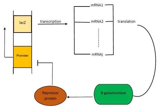
In this paper, we construct a discrete time delay Lac operon model with nonlinear degradation rate for mRNA, resulting from the interaction among several identical mRNA pieces. By taking a discrete time delay as bifurcation parameter, we investigate the nonlinear dynamical behaviour arising from the model, using mathematical tools such as stability and bifurcation theory. Firstly, we discuss the existence and uniqueness of the equilibrium for this system and investigate the effect of discrete delay on its dynamical behaviour. Absence or limited delay causes the system to have a stable equilibrium, which changes into a Hopf point producing oscillations if time delay is increased. These sustained oscillation are shown to be present only if the nonlinear degradation rate for mRNA satisfies specific conditions. The direction of the Hopf bifurcation giving rise to such oscillations is also determined, via the use of the so-called multiple time scales technique. Finally, numerical simulations are shown to validate and expand the theoretical analysis. Overall, our findings suggest that the degree of nonlinearity of the model can be used as a control parameter for the stabilisation of the system.

Keywords:

Citation: Zenab Alrikaby, Xia Liu, Tonghua Zhang, Federico Frascoli. Stability and Hopf bifurcation analysis for a Lac operon model with nonlinear degradation rate and time delay[J]. Mathematical Biosciences and Engineering, 2019, 16(4): 1729-1749. doi: 10.3934/mbe.2019083

Related Papers:

[1]	Leon J. van Ruiten, Thomas Hartmann . The spatial turn and the scenario approach in flood risk management—Implementing the European Floods Directive in the Netherlands. AIMS Environmental Science, 2016, 3(4): 697-713. doi: 10.3934/environsci.2016.4.697
[2]	Gene T. Señeris . Nabaoy River Watershed potential impact to flooding using Geographic Information System remote sensing. AIMS Environmental Science, 2022, 9(3): 381-402. doi: 10.3934/environsci.2022024
[3]	G Mathias Kondolf, Pilar Lopez-Llompart . National-local land-use conflicts in floodways of the Mississippi River system. AIMS Environmental Science, 2018, 5(1): 47-63. doi: 10.3934/environsci.2018.1.47
[4]	Vijendra Kumar, Kul Vaibhav Sharma, Nikunj K. Mangukiya, Deepak Kumar Tiwari, Preeti Vijay Ramkar, Upaka Rathnayake . Machine learning applications in flood forecasting and predictions, challenges, and way-out in the perspective of changing environment. AIMS Environmental Science, 2025, 12(1): 72-105. doi: 10.3934/environsci.2025004
[5]	Said Qasim, Mohammad Qasim, Rajendra Prasad Shrestha, Amir Nawaz Khan . An assessment of flood vulnerability in Khyber Pukhtunkhwa province of Pakistan. AIMS Environmental Science, 2017, 4(2): 206-216. doi: 10.3934/environsci.2017.2.206
[6]	Ronak P. Chaudhari, Shantanu R. Thorat, Darshan J. Mehta, Sahita I. Waikhom, Vipinkumar G. Yadav, Vijendra Kumar . Comparison of soft-computing techniques: Data-driven models for flood forecasting. AIMS Environmental Science, 2024, 11(5): 741-758. doi: 10.3934/environsci.2024037
[7]	RAHMOUN Ibrahim, BENMAMAR Saâdia, RABEHI Mohamed . Comparison between different Intensities of Rainfall to identify overflow points in a combined sewer system using Storm Water Management Model. AIMS Environmental Science, 2022, 9(5): 573-592. doi: 10.3934/environsci.2022034
[8]	Kitipol Nualtong, Ronnason Chinram, Piyawan Khwanmuang, Sukrit Kirtsaeng, Thammarat Panityakul . An efficiency dynamic seasonal regression forecasting technique for high variation of water level in Yom River Basin of Thailand. AIMS Environmental Science, 2021, 8(4): 283-303. doi: 10.3934/environsci.2021019
[9]	Finu Shrestha, Kabir Uddin, Sudan Bikash Maharjan, Samjwal Ratna Bajracharya . Application of remote sensing and GIS in environmental monitoring in the Hindu Kush Himalayan region. AIMS Environmental Science, 2016, 3(4): 646-662. doi: 10.3934/environsci.2016.4.646
[10]	Ignazio Mongelli, Michalis Vousdoukas, Luc Feyen, Antonio Soria, Juan-Carlos Ciscar . Long-term economic impacts of coastal floods in Europe: a probabilistic analysis. AIMS Environmental Science, 2023, 10(5): 593-608. doi: 10.3934/environsci.2023033

Abstract

1. Introduction

In 1960, Opial ^[12] established the following inequality:

Theorem A Suppose $f\in C^{1}[0, h]$ satisfies $f(0) = f(h) = 0$ and $f(x) > 0$ for all $x\in (0, h).$ Then the inequality holds

$\begin{align} \int_{0}^h\left|f(x)f'(x)\right|dx\leq\frac{h}{4}\int_{0}^{h}(f'(x))^{2}dx, \end{align}$

(1.1)

where this constant $h/4$ is best possible.

Many generalizations and extensions of Opial's inequality were established ^{[2,4,5,6,7,8,9,10,11,15,16,17,18,19]}. For an extensive survey on these inequalities, see ^[13]. Opial's inequality and its generalizations and extensions play a fundamental role in the ordinary and partial differential equations as well as difference equation ^{[2,3,4,6,7,9,10,11,17]}. In particular, Agarwal and Pang ^[3] proved the following Opial-Wirtinger's type inequalities.

Theorem B Let $\lambda\geq 1$ be a given real number, and let $p(t)$ be a nonnegative and continuous function on $[0, a]$ . Further, let $x(t)$ be an absolutely continuous function on $[0, a]$ , with $x(0) = x(a) = 0$ . Then

$\begin{align} \int_{0}^{a}p(t)|x(t)|^{\lambda}dt\leq\frac{1}{2}\int_{0}^{a}[t(a-t)]^{(\lambda-1)/2}p(t)dt\int_{0}^{a}\left|x'(t) \right|^{\lambda}dt. \end{align}$

(1.2)

The first aim of the present paper is to establish Opial-Wirtinger's type inequalities involving Katugampola conformable partial derivatives and $\alpha$ -conformable integrals (see Section 2). Our result is given in the following theorem, which is a generalization of (1.2).

Theorem 1.1 Let $\lambda\geq 1$ be a real number and $\alpha\in (0, 1]$ , and let $p(s, t)$ be a nonnegative and continuous functions on $[0, a]\times [0, b]$ . Further, let $x(s, t)$ be an absolutely continuous function and Katugampola partial derivable on $[0, a]\times [0, b]$ , with $x(s, 0) = x(0, t) = x(0, 0) = 0$ and $x(a, b) = x(a, t) = x(s, b) = 0$ . If $p > 1,$ $\frac{1}{p}+\frac{1}{q} = 1$ Then

$\int_{0}^{a}\int_{0}^{b}p(s, t)|x(s, t)|^{\lambda}d_{\alpha}sd_{\alpha}t\leq\frac{p+q}{pq} \left(\frac{1}{\alpha^{2}}\right)^{\lambda-1}\left(\int_{0}^{a}\int_{0}^{b}\Gamma_{abpq\lambda\alpha}(s, t)\cdot p(s, t)d_{\alpha}sd_{\alpha}t\right)$

$\begin{align} \times\int_{0}^{a}\int_{0}^{b}\left|\frac{\partial^{2}}{\partial s\partial t}(x)_{\alpha^{2}}(s, t)\right|^{\lambda}d_{\alpha}sd_{\alpha}t, \end{align}$

(1.3)

where

$\Gamma_{abpq\lambda\alpha}(s, t) = \left\{(st)^{1/p}[(a-s)(b-t)]^{1/q}\right\}^{\alpha(\lambda-1)}.$

Remark 1.1 Let $x(s, t)$ reduce to $s(t)$ and with suitable modifications, and $p = q = 2$ and $\alpha = 1$ , (1.3) become (1.2).

Theorem C Let $\lambda\geq 1$ be a given real number, and let $p(t)$ be a nonnegative and continuous function on $[0, a]$ . Further, let $x(t)$ be an absolutely continuous function on $[0, a]$ , with $x(0) = x(a) = 0$ . Then

$\begin{align} \int_{0}^{a}p(t)|x(t)|^{\lambda}dt\leq\frac{1}{2}\left(\frac{a}{2} \right)^{\lambda-1}\left(\int_{0}^{a}p(t)dt\right)\int_{0}^{a}\left|x'(t)\right|^{\lambda}dt. \end{align}$

(1.4)

Another aim of this paper is to establish the following inequality involving Katugampola conformable partial derivatives and $\alpha$ -conformable integrals. Our result is given in the following theorem.

Theorem 1.2 Let $j = 1, 2$ and $\lambda\geq 1$ be a real number, and let $p_{j}(s, t)$ be a nonnegative and continuous functions on $[0, a]\times [0, b]$ . Further, let $x_{j}(s, t)$ be an absolutely continuous function and Katugampola partial derivable on $[0, a]\times [0, b]$ , with $x_{j}(s, 0) = x_{j}(0, t) = x_{j}(0, 0) = 0$ and $x_{j}(a, b) = x_{j}(a, t) = x_{j}(s, b) = 0$ . Then for $\alpha\in(0, 1]$

$\int_{0}^{a}\int_{0}^{b}\left(p_{1}(s, t)|x_{1}(s, t)|^{\lambda}+p_{2}(s, t)|x_{2}(s, t)|^{\lambda}\right)d_{\alpha}sd_{\alpha}t\; \; \; \; \; \; \; \; \; \; \; \; \; \; \; \; \; \; \; \; \; \; \; \; \; \; \; \; \; \; \; \; \; \; \; \; \; \; \; \; \; \; \; \; \; \; \; \; \; \; \; \; \; \; \; \; \; \; \; \;$

$\leq\frac{1}{2^{\lambda}}\left(\frac{1}{\alpha^{2}}\right)^{\lambda-1}\Bigg[\left(\int_{0}^{a}\int_{0}^{b}(st)^{\alpha(\lambda-1)}p_{1}(s, t) d_{\alpha}sd_{\alpha}t\right)\int_{0}^{a}\int_{0}^{b}\left|\frac{\partial^{2}}{\partial s\partial t}(x_{1})_{\alpha^{2}}(s, t)\right|^{\lambda} d_{\alpha}sd_{\alpha}t$

$\begin{align} +\left(\int_{0}^{a}\int_{0}^{b}(st)^{\alpha(\lambda-1)}p_{2}(s, t)d_{\alpha}sd_{\alpha}t\right)\int_{0}^{a}\int_{0}^{b}\left|\frac{\partial^{2}}{\partial s\partial t}(x_{2})_{\alpha^{2}}(s, t)\right|^{\lambda}d_{\alpha}sd_{\alpha}t\Bigg]. \end{align}$

(1.5)

2. Katugampola conformable partial derivatives

Here, let's recall the well-known Katugampola derivative formulation of conformable derivative of order for $\alpha\in(0, 1]$ and $t\in[0, \infty)$ , given by

$\begin{align} {\cal D}_{\alpha}(f)(t) = \lim\limits_{\varepsilon\rightarrow 0}\frac{f(te^{\varepsilon t^{-\alpha}})-f(t)}{\varepsilon}, \end{align}$

(2.1)

and

$\begin{align} {\cal D}_{\alpha}(f)(0) = \lim\limits_{t\rightarrow 0}D_{\alpha}(f)(t), \end{align}$

(2.2)

provided the limits exist. If $f$ is fully differentiable at $t$ , then

${\cal D}_{\alpha}(f)(t) = t^{1-\alpha}\frac{df}{dt}(t).$

A function $f$ is $\alpha$ -differentiable at a point $t\geq 0$ , if the limits in (2.1) and (2.2) exist and are finite. Inspired by this, we propose a new concept of $\alpha$ -conformable partial derivative. In the way of (1.4), $\alpha$ -conformable partial derivative is defined in as follows:

Definition 2.1 ^[20] ( $\alpha$ -conformable partial derivative) Let $\alpha\in (0, 1]$ and $s, t\in[0, \infty)$ . Suppose $f(s, t)$ is a continuous function and partial derivable, the $\alpha$ -conformable partial derivative at a point $s\geq 0$ , denoted by $\frac{\partial}{\partial s}(f)_{\alpha}(s, t)$ , defined by

$\begin{align} \frac{\partial}{\partial s}(f)_{\alpha}(s, t) = \lim\limits_{\varepsilon\rightarrow 0}\frac{f(se^{\varepsilon s^{-\alpha}}, t)-f(s, t)} {\varepsilon}, \end{align}$

(2.3)

provided the limits exist, and call $\alpha$ -conformable partial derivable.

Recently, Katugampola conformable partial derivative is defined in as follows:

Definition 2.2 ^[20] (Katugampola conformable partial derivatives) Let $\alpha\in (0, 1]$ and $s, t\in[0, \infty)$ . Suppose $f(s, t)$ and $\frac{\partial}{\partial s}(f)_{\alpha}(s, t)$ are continuous functions and partial derivable, the Katugampola conformable partial derivative, denoted by $\frac{\partial^{2}}{\partial s\partial t}(f)_{\alpha^{2}}(s, t)$ , defined by

$\begin{align} \frac{\partial^{2}}{\partial s\partial t}(f)_{\alpha^{2}}(s, t) = \lim\limits_{\varepsilon\rightarrow 0}\frac{\frac{\partial}{\partial s}(f)_{\alpha}(s, te^{\varepsilon t^{-\alpha}})-\frac{\partial}{\partial s}(f)_{\alpha}(s, t)}{\varepsilon}, \end{align}$

(2.4)

provided the limits exist, and call Katugampola conformable partial derivable.

Definition 2.3 ^[20] ( $\alpha$ -conformable integral) Let $\alpha\in (0, 1]$ , $0\leq a < b$ and $0\leq c < d$ . A function $f(x, y):[a, b]\times[c, d]\rightarrow {\Bbb R}$ is $\alpha$ -conformable integrable, if the integral

$\begin{align} \int_{a}^{b}\int_{c}^{d}f(x, y)d_{\alpha}xd_{\alpha}y: = \int_{a}^{b}\int_{c}^{d} (xy)^{\alpha-1}f(x, y)dxdy \end{align}$

(2.5)

exists and is finite.

3. Main results

Theorem 3.1 Let $\lambda\geq 1$ be a real number and $\alpha\in (0, 1]$ , and let $p(s, t)$ be a nonnegative and continuous functions on $[0, a]\times [0, b]$ . Further, let $x(s, t)$ be an absolutely continuous function and Katugampola partial derivable on $[0, a]\times [0, b]$ , with $x(s, 0) = x(0, t) = x(0, 0) = 0$ and $x(a, b) = x(a, t) = x(s, b) = 0$ . If $p > 1,$ $\frac{1}{p}+\frac{1}{q} = 1$ Then

$\begin{align} \times\int_{0}^{a}\int_{0}^{b}\left|\frac{\partial^{2}}{\partial s\partial t}(x)_{\alpha^{2}}(s, t)\right|^{\lambda}d_{\alpha}sd_{\alpha}t, \end{align}$

(3.1)

where

$\Gamma_{abpq\lambda\alpha}(s, t) = \left\{(st)^{1/p}[(a-s)(b-t)]^{1/q}\right\}^{\alpha(\lambda-1)}.$

Proof From (2.4) and (2.5), we have

$x(s, t) = \int_{0}^{s}\int_{0}^{t}\frac{\partial^{2}}{\partial s\partial t}(x)_{\alpha^{2}}(s, t)d_{\alpha}sd_{\alpha}t.$

By using Hölder's inequality with indices $\lambda$ and $\lambda/(\lambda-1)$ , we have

$|x(s, t)|^{\lambda/p}\leq \left[\left(\int_{0}^{s}\int_{0}^{t}\left|\frac{\partial^{2}}{\partial s\partial t} (x)_{\alpha^{2}}(s, t)\right|d_{\alpha}sd_{\alpha}t\right)^{\lambda}\right]^{1/p}\; \; \; \; \; \; \; \; \; \; \; \; \; \; \; \; \; \; \; \; \; \; \; \; \; \; \; \; \; \; \; \; \; \; \; \;$

$\begin{align} \leq\left(\frac{1}{\alpha^{2}}(st)^{\alpha}\right)^{(\lambda-1)/p}\left(\int_{0}^{s}\int_{0}^{t}\left|\frac{\partial^{2}}{\partial s\partial t}(x)_{\alpha^{2}}(s, t)\right|^{\lambda}d_{\alpha}sd_{\alpha}t\right)^{1/p}. \end{align}$

(3.2)

Similarly, from

$x(s, t) = \int_{s}^{a}\int_{t}^{b}\frac{\partial^{2}}{\partial s\partial t}(x)_{\alpha^{2}}(s, t)d_{\alpha}sd_{\alpha}t,$

we obtain

$\begin{align} |x(s, t)|^{\lambda/q}\leq \left(\frac{1}{\alpha^{2}}[(a-s)(b-t)]^{\alpha}\right)^{(\lambda-1)/q} \left(\int_{s}^{a}\int_{t}^{b}\left|\frac{\partial^{q}}{\partial s\partial t}(x)_{\alpha^{2}}(s, t)\right|^{\lambda}d_{\alpha}sd_{\alpha}t\right)^{1/q}. \end{align}$

(3.3)

Now a multiplication of (3.2) and (3.3), and by using the well-known Young inequality gives

$\begin{eqnarray*} |x(s, t)|^{\lambda}&\leq &\left(\frac{1}{\alpha^{2}}\right)^{\lambda-1}\cdot\Gamma_{abpq\lambda\alpha}(s, t)\cdot\left(\int_{0}^{s}\int_{0}^{t} \left|\frac{\partial^{2}}{\partial s\partial t}(x)_{\alpha^{2}}(s, t)\right|^{\lambda}d_{\alpha}sd_{\alpha}t\right)^{1/p}\\ &\times&\left(\int_{s}^{a}\int_{t}^{b}\left|\frac{\partial^{2}}{\partial s\partial t}(x)_{\alpha^{2}}(s, t)\right|^{\lambda}d_{\alpha}sd_{\alpha}t\right)^{1/q}\\ &\leq &\left(\frac{1}{\alpha^{2}}\right)^{\lambda-1}\cdot\Gamma_{abpq\lambda\alpha}(s, t)\cdot\Bigg(\frac{1}{p}\int_{0}^{s}\int_{0}^{t}\left|\frac{\partial^{2}}{\partial s\partial t}(x)_{\alpha^{2}}(s, t)\right|^{\lambda}d_{\alpha}sd_{\alpha}t\\ &+&\frac{1}{q}\int_{s}^{a}\int_{t}^{b}\left|\frac{\partial^{2}}{\partial s\partial t}(x)_{\alpha^{2}}(s, t)\right|^{\lambda}d_{\alpha}sd_{\alpha}t\Bigg) \end{eqnarray*}$

$\begin{align} \; \; \; \; \; \; \; \; \; \; = \frac{p+q}{pq}\left(\frac{1}{\alpha^{2}}\right)^{\lambda-1}\cdot\Gamma_{abpq\lambda\alpha}(s, t)\int_{0}^{a}\int_{0}^{b}\left|\frac{\partial^{2}}{\partial s\partial t}(x)_{\alpha^{2}}(s, t)\right|^{\lambda}d_{\alpha}sd_{\alpha}t, \end{align}$

(3.4)

where

$\Gamma_{abpq\lambda\alpha}(s, t) = \Big\{(st)^{1/p}[(a-s)(b-t)]^{1/q}\Big\} ^{\alpha(\lambda-1)}.$

Multiplying the both sides of (3.4) by $p(s, t)$ and $\alpha$ –conformable integrating both sides over $t$ from $0$ to $b$ first and then integrating the resulting inequality over $s$ from $0$ to $a$ , we obtain

$\int_{0}^{a}\int_{0}^{b}p(s, t)|x(s, t)|^{\lambda}d_{\alpha}sd_{\alpha}t\; \; \; \; \; \; \; \; \; \; \; \; \; \; \; \; \; \; \; \; \; \; \; \; \; \; \; \; \; \; \; \; \; \; \; \; \; \; \; \; \; \; \; \; \; \; \; \; \; \; \; \; \; \; \; \; \; \; \; \; \; \; \; \; \; \; \; \; \; \; \; \; \; \; \; \; \; \; \; \; \; \; \; \; \; \; \; \; \; \; \; \; \; \; \; \;$

$\leq\frac{p+q}{pq}\left(\frac{1}{\alpha^{2}}\right)^{\lambda-1}\cdot\int_{0}^{a}\int_{0}^{b}\Gamma_{abpq\lambda\alpha}(s, t)\cdot p(s, t)\left(\int_{0}^{a}\int_{0}^{b}\left|\frac{\partial^{2}}{\partial s\partial t}(x)_{\alpha^{2}}(s, t)\right|^{\lambda}d_{\alpha}sd_{\alpha}t\right)d_{\alpha}sd_{\alpha}t$

$= \frac{p+q}{pq}\left(\frac{1}{\alpha^{2}}\right)^{\lambda-1}\cdot\left(\int_{0}^{a}\int_{0}^{b}\Gamma_{abpq\lambda\alpha}(s, t)\cdot p(s, t)d_{\alpha}sd_{\alpha}t\right)\int_{0}^{a}\int_{0}^{b}\left|\frac{\partial^{2}}{\partial s\partial t}(x)_{\alpha^{2}}(s, t)\right|^{\lambda}d_{\alpha}sd_{\alpha}t.$

This completes the proof.

Remark 3.1 Let $x(s, t)$ reduce to $s(t)$ and with suitable modifications, (3.1) becomes the following result.

$\begin{align} \int_{0}^{a}p(t)|x(t)|^{\lambda}d_{\alpha}t\leq\frac{p+q}{pq}\left(\frac{1}{\alpha^{2}}\right)^{\lambda-1}\cdot\int_{0}^{a} \Gamma_{apq\lambda\alpha}(t)p(t)d_{\alpha}t\int_{0}^{a}\left|{\cal D}_{\alpha}(x)(t) \right|^{\lambda}d_{\alpha}t, \end{align}$

(3.5)

where ${\cal D}_{\alpha}(x)(t)$ is Katugampola derivative (2.1) stated in the introduction, and

$\Gamma_{apq\lambda\alpha}(t) = \Big\{t^{1/p}(a-t)^{1/q}\Big\} ^{\alpha(\lambda-1)}.$

Putting $p = q = 2$ and $\alpha = 1$ in (3.5), (3.5) becomes inequality (1.2) established by Agarwal and Pang ^[3] stated in the introduction.

Taking for $\alpha = 1$ , $p = q = 2$ and $p(s, t) = {\rm constant}$ in (3.1), we have the following interesting result.

$\int_{0}^{a}\int_{0}^{b}|x(s, t)|^{\lambda}dsdt\leq \frac{1}{2}(ab)^{\lambda}\left[B\left(\frac{\lambda+1}{2}, \frac{\lambda+1}{2}\right)\right] ^{2}\int_{0}^{a}\int_{0}^{b}\left|\frac{\partial^{2}}{\partial s\partial t}x(s, t)\right|^{\lambda}dsdt,$

where $B$ is the Beta function.

Theorem 3.2 Let $j = 1, 2$ and $\lambda\geq 1$ be a real number, and let $p_{j}(s, t)$ be a nonnegative and continuous functions on $[0, a]\times [0, b]$ . Further, let $x_{j}(s, t)$ be an absolutely continuous function and Katugampola partial derivable on $[0, a]\times [0, b]$ , with $x_{j}(s, 0) = x_{j}(0, t) = x_{j}(0, 0) = 0$ and $x_{j}(a, b) = x_{j}(a, t) = x_{j}(s, b) = 0$ . Then for $\alpha\in(0, 1]$

(3.6)

Proof Because

$x_{1}(s, t) = \int_{0}^{s}\int_{0}^{t}\frac{\partial^{2}}{\partial s\partial t}(x_{1})_{\alpha^{2}}(s, t)d_{\alpha}sd_{\alpha}t = \int_{s}^{a}\int_{t}^{b}\frac{\partial^{2}}{\partial s\partial t}(x_{1})_{\alpha^{2}}(s, t)d_{\alpha}sd_{\alpha}t.$

Hence

$|x_{1}(s, t)|\leq\frac{1}{2}\int_{0}^{a}\int_{0}^{b}\left|\frac{\partial^{2}}{\partial s\partial t}(x_{1})_{\alpha^{2}}(s, t)\right|d_{\alpha}sd_{\alpha}t.$

By Hölder's inequality with indices $\lambda$ and $\lambda/(\lambda-1)$ , it follows that

$p_{1}(s, t)|x_{1}(s, t)|^{\lambda}\leq\frac{1}{2^{\lambda}}p_{1}(s, t)\left(\int_{0}^{a}\int_{0}^{b}\left|\frac{\partial^{2}}{\partial s\partial t} (x_{1})_{\alpha^{2}}(s, t)\right|d_{\alpha}sd_{\alpha}t \right)^{\lambda}\; \; \; \; \; \; \; \; \; \; \; \; \; \; \; \; \; \; \; \; \; \; \; \; \; \; \; \; \; \; \; \; \; \; \; \; \; \;$

$\begin{align} \; \; \; \; \; \; \; \; \; \; \; \; \; \; \; \leq\frac{1}{2^{\lambda}}\left(\frac{1}{\alpha^{2}}\right)^{\lambda-1}(st)^{\alpha(\lambda-1)}p_{1}(s, t)\int_{0}^{a}\int_{0}^{b}\left|\frac{\partial^{2}}{\partial s\partial t}(x_{1})_{\alpha^{2}}(s, t)\right|^{\lambda}d_{\alpha}sd_{\alpha}t, \end{align}$

(3.7)

Similarly

$\begin{align} p_{2}(s, t)|x_{2}(s, t)|^{\lambda}\leq\frac{1}{2^{\lambda}}\left(\frac{1}{\alpha^{2}}\right)^{\lambda-1}(st)^{\alpha(\lambda-1)}p_{2}(s, t)\int_{0}^{a}\int_{0}^{b} \left|\frac{\partial^{2}}{\partial s\partial t}(x_{2})_{\alpha^{2}}(s, t)\right|^{\lambda}d_{\alpha}sd_{\alpha}t, \end{align}$

(3.8)

Taking the sum of (3.7) and (3.8) and $\alpha$ -integrating the resulting inequalities over $t$ from $0$ to $b$ first and then over $s$ from $0$ to $a$ , we obtain

$\int_{0}^{a}\int_{0}^{b}\left(p_{1}(s, t)|x_{1}(s, t)|^{\lambda}+p_{2}(s, t)|x_{2}(s, t)|^{\lambda}\right)d_{\alpha}s d_{\alpha}t\; \; \; \; \; \; \; \; \; \; \; \; \; \; \; \; \; \; \; \; \; \; \; \; \; \; \; \; \; \; \; \; \; \; \; \; \; \; \; \; \; \; \; \; \; \; \; \; \; \; \; \; \; \; \;$

$\begin{eqnarray*} &\leq&\frac{1}{2^{\lambda}}\left(\frac{1}{\alpha^{2}}\right)^{\lambda-1}\Bigg\{\int_{0}^{a}\int_{0}^{b}\left((st)^{\alpha(\lambda-1)}p_{1}(s, t) \int_{0}^{a}\int_{0}^{b}\left|\frac{\partial^{2}}{\partial s\partial t}(x_{1})_{\alpha^{2}}(s, t)\right|^{\lambda}d_{\alpha}sd_{\alpha}t\right)d_{\alpha}sd_{\alpha}t\\ &+&\int_{0}^{a}\int_{0}^{b}\left((st)^{\alpha(\lambda-1)}p_{2}(s, t)\int_{0}^{a}\int_{0}^{b}\left|\frac{\partial^{2}}{\partial s\partial t}(x_{2})_{\alpha^{2}}(s, t)\right|^{\lambda}d_{\alpha}sd_{\alpha}t\right)d_{\alpha}sd_{\alpha}t\Bigg\}\\ & = &\frac{1}{2^{\lambda}}\left(\frac{1}{\alpha^{2}}\right)^{\lambda-1}\Bigg[\left(\int_{0}^{a}\int_{0}^{b}(st)^{\alpha(\lambda-1)}p_{1}(s, t) d_{\alpha}sd_{\alpha}t\right)\int_{0}^{a}\int_{0}^{b}\left|\frac{\partial^{2}}{\partial s\partial t}(x_{1})_{\alpha^{2}}(s, t)\right|^{\lambda} d_{\alpha}sd_{\alpha}t\\ &+&\left(\int_{0}^{a}\int_{0}^{b}(st)^{\alpha(\lambda-1)}p_{2}(s, t)d_{\alpha}sd_{\alpha}t\right)\int_{0}^{a}\int_{0}^{b}\left|\frac{\partial^{2}}{\partial s\partial t}(x_{2})_{\alpha^{2}}(s, t)\right|^{\lambda}d_{\alpha}sd_{\alpha}t\Bigg]. \end{eqnarray*}$

Remark 3.2 Taking for $x_{1}(s, t) = x_{2}(s, t) = x(s, t)$ and $p_{1}(s, t) = p_{2}(s, t) = p(s, t)$ in (3.6), (3.6) changes to the following inequality.

$\int_{0}^{a}\int_{0}^{b}p(s, t)|x(s, t)|^{\lambda}d_{\alpha}sd_{\alpha}t\leq\frac{1}{2^{\lambda}}\left(\frac{1} {\alpha^{2}}\right)^{\lambda-1}\; \; \; \; \; \; \; \; \; \; \; \; \; \; \; \; \; \; \; \; \; \; \; \; \; \; \; \; \; \; \; \; \; \; \; \; \; \;$

$\begin{align} \times\left(\int_{0}^{a}\int_{0}^{b}(st)^{\alpha(\lambda-1)}p(s, t) d_{\alpha}sd_{\alpha}t\right) \int_{0}^{a}\int_{0}^{b}\left|\frac{\partial^{2}}{\partial s\partial t} (x)_{\alpha^{2}}(s, t)\right|^{\lambda}d_{\alpha}sd_{\alpha}t. \end{align}$

(3.9)

Putting $\alpha = 1$ in (3.9), we have

$\begin{align} \int_{0}^{a}\int_{0}^{b}p(s, t)|x(s, t)|^{\lambda}dsdt\leq\frac{1}{2^{\lambda}}\left(\int_{0}^{a}\int_{0}^{b}(st)^{\lambda-1}p(s, t) dsdt\right)\int_{0}^{a}\int_{0}^{b}\left|\frac{\partial^{2}}{\partial s\partial t} x(s, t)\right|^{\lambda}dsdt. \end{align}$

(3.10)

Let $x(s, t)$ reduce to $s(t)$ and with suitable modifications, and $\lambda = 1$ , (2.10) becomes the following result.

$\begin{align} \int_{0}^{a}p(t)|x(t)|dt\leq\frac{1}{2}\left(\int_{0}^{a}p(t)dt\right)\int_{0}^{a}\left|x'(t)\right|dt. \end{align}$

(3.11)

This is just a new inequality established by Agarwal and Pang ^[4]. For $\lambda = 2$ the inequality (3.11) has appear in the work of Traple ^[14], Pachpatte ^[13] proved it for $\lambda = 2m$ ( $m\geq 1$ an integer).

Remark 3.3 Let $x_{j}(s, t)$ reduce to $x_{j}(t)$ ( $j = 1, 2$ ) and $p_{j}(s, t)$ reduce to $p_{j}(t)$ ( $j = 1, 2$ ) with suitable modifications, (3.6) becomes the following interesting result.

$\int_{0}^{a}\left(p_{1}(t)|x_{1}(t)|^{\lambda}+p_{2}(t)|x_{2}(t)|^{\lambda}\right)d_{\alpha}t\leq\frac{1}{2^{\lambda}}\left(\frac{1} {\alpha^{2}}\right)^{\lambda-1}\Bigg[\left(\int_{0}^{a}t^{\alpha(\lambda-1)}p_{1}(t)d_{\alpha}t\right)\int_{0}^{a}\left|{\cal D }_{\alpha}(x'_{1})(t)\right|^{\lambda} d_{\alpha}t$

$\begin{align} \; \; \; \; \; \; \; \; \; \; \; \; \; \; \; \; \; \; \; \; \; \; \; \; \; \; \; \; \; \; \; \; \; \; \; \; \; \; \; \; \; \; \; \; +\left(\int_{0}^{a}t^{\alpha(\lambda-1)}p_{2}(t)d_{\alpha}t\right)\int_{0}^{a}\left|{\cal D}_{\alpha}(x'_{2})(t)\right|^{\lambda}d_{\alpha}t\Bigg]. \end{align}$

(3.12)

Putting $\lambda = 1$ and $\alpha = 1$ in (3.12), we have the following interesting result.

$\int_{0}^{a}\left(p_{1}(t)|x_{1}(t)|+p_{2}(t)|x_{2}(t)|\right)dt\leq\frac{1}{2}\Bigg(\int_{0}^{a}p_{1}(t)dt\int_{0}^{a}\left|x'_{1}(t)\right| dt+\int_{0}^{a}p_{2}(t)dt\int_{0}^{a}\left|x'_{2}(t)\right|dt\Bigg).$

Finally, we give an example to verify the effectiveness of the new inequalities. Estimate the following double integrals:

$\int_{0}^{1}\int_{0}^{1}\Big[st(s-1)(t-1)\Big]^{\lambda}dsdt,$

where $\lambda\geq 1$ .

Let $x_{1}(s,t)=x_{2}(s,t)= x(s, t) = st(s-1)(t-1)$ , $p_{1}(s,t)=p_{2}(s,t)= p(s, t) = (st)^{1-\alpha}$ , $a = b = 1$ and $0 < \alpha\leq 1$ , and by using Theorem 3.2, we obtain

$\int_{0}^{1}\int_{0}^{1}\Big[st(s-1)(t-1)\Big]^{\lambda}dsdt\; \; \; \; \; \; \; \; \; \; \; \; \; \; \; \; \; \; \; \; \; \; \; \; \; \; \; \; \; \; \; \; \; \; \; \; \; \; \; \; \; \; \; \; \; \; \; \; \; \; \; \; \; \; \; \; \; \; \; \; \; \; \; \; \; \; \; \; \; \; \; \; \; \; \; \; \; \; \; \; \; \; \; \; \;$

$\begin{eqnarray*} & = &\int_{0}^{1}\int_{0}^{1}p(s, t) \left|x(s, t)\right|^{\lambda}d_{\alpha}sd_{\alpha}t\\ &\leq&\frac{1}{2^{\lambda}}\left(\frac{1} {\alpha^{2}}\right)^{\lambda-1}\left(\int_{0}^{1}\int_{0}^{1}(st)^{\alpha(\lambda-1)}p(s, t) d_{\alpha}sd_{\alpha}t\right) \int_{0}^{1}\int_{0}^{1}\left|\frac{\partial^{2}}{\partial s\partial t} (x)_{\alpha^{2}}(s, t)\right|^{\lambda}d_{\alpha}sd_{\alpha}t\\ & = &\frac{1}{2^{\lambda}}\left(\frac{1} {\alpha^{2}}\right)^{\lambda-1}\left(\frac{1}{\alpha(\lambda-1)+1}\right)^{2} \int_{0}^{1}\int_{0}^{1}\Big[(2s-1)(2t-1)\Big]^{\lambda}(st)^{\alpha-1}dsdt\\ & = &\frac{1}{2^{\lambda}}\left(\frac{1} {\alpha^{2}}\right)^{\lambda-1}\left(\frac{1}{\alpha(\lambda-1)+1}\right)^{2} \left(\frac{1}{2^{\alpha-1}}\int_{-1}^{1}t^{\lambda}\frac{1}{(t+1)^{1-\alpha}}dt\right)^{2}\\ &\leq&\frac{1}{2^{\lambda}}\left(\frac{1} {\alpha^{2}}\right)^{\lambda-1}\left(\frac{1}{\alpha(\lambda-1)+1}\right)^{2} \left(\frac{1}{2^{\alpha-1}}\frac{2^{\alpha}}{\alpha}\right)^{2}\\ & = &\frac{2^{2-\lambda}}{\alpha^{2\lambda}\left(\alpha(\lambda-1)+1\right)^{2}}. \end{eqnarray*}$

4. Conclusions

We have introduced a general version of Opial-Wirtinger's type integral inequality for the Katugampola partial derivatives. The established results are generalization of some existing Opial type integral inequalities in the previous published studies. For further investigations we propose to consider the Opial-Wirtinger's type inequalities for other partial derivatives.

Acknowledgments

I would like to thank that research is supported by National Natural Science Foundation of China(11471334, 10971205).

Conflict of interest

The author declares no conflicts of interest.

References

[1]	B. Goodwin, Oscillatory behaviour in enzymatic control process, Adv. Enzyme Regul., 3 (1965), 425–438.
[2]	S. Busenberg and J. Mahaffy, Interaction of spatial diffusion and delays in models of genetic control by repression, J. Math. Biol., 22 (1985), 313–333.
[3]	J. Mahaffy and C. Pao, Models of genetic control by repression with time delays and spatial effects, J. Math. Biol., 20 (1984), 39–57.
[4]	M. Monk, Oscillatory expression of Hes1, p53, and NF-k B driven by transcription time delays, Curr. Biol., 13 (2003), 1409–1413.
[5]	S. Nikolov, J. Vera, V. Kotev, et al., Dynamic properties of a delayed protein cross talk model, BioSystems, 91 (2008), 483–500.
[6]	Y. Song, X. Cao and T. Zhang, Bistability and delay-induced stability switches in a cancer network with the regulation of microRNA, Commun. Nonlinear Sci. Numer. Simul., 54 (2018), 302–319.
[7]	N. Yildirim, M. Santillan and D. Horike, Dynamics and bi-stability in a reduced model of the lac operon, Chaos, 14 (2004), 279–291.
[8]	N. Yildirim and M. Mackey, Feedback regulation in the Lactose operon: a Mathematical modeling study and comparison with experimental data, Biophys. J., 84 (2003), 2841–2851.
[9]	A. Verdugo, Dynamics of gene networks with time delays, Ph.D thesis, Cornell university, USA, 2009.
[10]	K. Wang, L. Wang, Z. Teng, et al., Stability and bifurcation of genetic regulatory networks with delays, Neurocomputing, 73 (2010), 2882–2892.
[11]	H. Zang, T. Zhang and Y. Zhang, Bifurcation analysis of a mathematical model for genetic regulatory network with time delays, Appl. Math. Comput., 260 (2015), 204–226.
[12]	M. B. Elowitz and S. Leibler, A synthetic oscillatory network of transcription regulators, Nature, 403 (2000), 335–338.
[13]	D. Liu, X. Chang, Z. Liu, et al., Bistability and Oscillations in Gene Regulation Mediated by Small Noncoding RNAs, PLoS ONE, 6 (2011), e17029.
[14]	H. Liu, F. Yan and Z. Liu, Oscillatory dynamics in a gene regulatory network mediated by small RNA with time delay, Nonlinear Dyn., 76 (2014), 147–159.
[15]	C. Sears and W. Garrett, Microbes, Microbiota and Colon Cancer, Nonlinear Dyn., 15 (2014), 317–328.
[16]	Q. Xie, T. Wanga, C. Zeng, et al., Predicting fluctuations-caused regime shifts in a time delayed dynamics of an invading species, Physica A, 493 (2018), 69–83.
[17]	C. Zeng, Q. Xie, T. Wang, et al., Stochastic ecological kinetics of regime shifts in a time-delayed lake eutrophication ecosystem, Ecosphere, 8 (2017), 1–34.
[18]	J. Zeng, C. Zeng, Q. Xie, et al., Different delays-induced regime shifts in a stochastic insect outbreak dynamics, Physica A, 462 (2016), 1273–1285.
[19]	C. Zeng and H. Wangb, Noise and large time delay: Accelerated catastrophic regime shifts in ecosystems, Ecol. Model., 233 (2012), 52–58.
[20]	C. Zeng, Q. Han, T. Yang, et al., Noise- and delay-induced regime shifts in an ecological system of vegetation, J. Stat. Mech., 10 (2013), P10017.
[21]	Q. Han, T. Yang, C. Zeng, et al., Impact of time delays on stochastic resonance in an ecological system describing vegetation, Physica A, 408 (2014), 96–105.
[22]	B. D. Aguda, Y. Kim, M. G. Piper-Hunter, et al., MicroRNA regulation of a cancer network: Consequences of the feedback loops involving miR-17-92, E2F, and Myc, PNAS, 105 (2008), 19678–19683.
[23]	S. Bernard, J. Belair and M. C. Macky, Sufficient conditions for stability of linear differential equations with distributed delay, Discrete Cont. Dyn-S B, 1 (2001), 233–256.
[24]	G. A. Calin, C Sevignani, C. D. Dumitru, et al., Human microRNA genes are frequently located at fragile sites and genomic regions involved in cancers, Proc. Natl. Acad. Sci. USA, 101 (2004), 2999–3004.
[25]	Y. Gao, B. Feng, S. Han, et al., The Roles of MicroRNA-141 in Human Cancers: From Diagnosis to Treatment, Cell Physiol. Biochem., 38 (2016), 427–448.
[26]	Y. Gao, B. Feng, L. Lu, et al., MiRNAs and E2F3: a complex network of reciprocal regulations in human cancers, Oncotarget, 8 (2017), 60624–60639.
[27]	I.V. Makunin, M. Pheasant, C. Simons, et al., Orthologous MicroRNA Genes Are Located in Cancer Associated Genomic Regions in Human and Mouse, PLoS ONE, 11 (2007), e1133.
[28]	F. Yan, H. Liu, J. Hao, et al., Dynamical Behaviors of Rb-E2F Pathway Including Negative Feedback Loops Involving miR449, PLoS ONE, 7 (2009), e43908.
[29]	Y. Peng and T. Zhang, Stability and Hopf bifurcation analysis of a gene expression model with diffusion and time delay, Abstr. Appl. Anal., 2014 (2014), 1–9.
[30]	H. Wang and J. Wang, Hopf-pitchfork bifurcation in a two-neuron system with discrete and distributed delays, Math, Meth, Appl, Sci., 38 (2015), 4967–4981.
[31]	A. Verdugo and R. Rand, Hopf bifurcation analysis for a model of genetic regulatory system with delay, Commun. Nonlinear Sci. Number. Simul., 13 (2008), 235–242.
[32]	J. Wei and C. Yu, Hopf bifurcation analysis in a model of oscillatory gene expression with delay, the Royal Society of Edinburgh, 139 (2009), 879–895.
[33]	X. Cao, Y. Song and T. Zhang, Hop bifurcation and delay induce Turing instability in a diffusive lac operon model, Int. J. Bifurcat. Chaos, 26 (2016), 1650–1667.
[34]	J. Yu and M. Peng, Local Hopf bifurcation analysis and global existence of periodic solutions in a gene expression model with delays, Nonlinear Dyn., 86 (2016), 245–256.
[35]	Y. A. Kuznetsov, Elements of Applied Bifurcation Theory, 3^rd edition, New York: Springer, 2004.
[36]	A. H. Nayfe, Order reduction of retarded nonlinear systems- the method of multiple scales versus center-manifold reduction, Nonlinear Dyn., 51 (2008), 483–500.
[37]	T. Zhang, Y. Song and H. Zang, The stability and Hopf bifurcation analysis of a gene expression model, J. Math. Anal. Appl., 395 (2012), 103–113.
[38]	L. Zheng, M. Chen and Q. Nie, External noise control in inherently stochastic biological systems, J. Math. Phys., 53 (2012), 115616.
[39]	R. Cruz, R. Perez-Carrasco, P. Guerrero, et al., Minimum Action Path Theory Reveals the Details of Stochastic Transitions Out of Oscillatory States, Phys. Rev. Lett., 120 (2018), 128102.
[40]	N. Guisoni, D. Monteoliva and L. Diambra, Promoters Architecture-Based Mechanism for Noise- Induced Oscillations in a Single-Gene Circuit, PLoS ONE, 11 (2016), e0151086.
[41]	B. Ingalls, Mathematical Modelling in Systems Biology: An Introduction, 1^st edition, Cambridge, MA, USA, 2013.
[42]	D. A. Potoyan and P. G. Wolynes, On the dephasing of genetic oscillators, PNAS, 6 (2014), 2391–2396.
[43]	F. Jacob, D. Perrin, C. Sanchez, et al., Lac operon: A Group of genes whose expression is coordinated by an operator, CR Biol., 250 (1960), 1727–1729.
[44]	S. Liu and L. Wang, Global stability of an HIV-1 model with distributed intracellular delays and a combination therapy, Math. Biosci. Eng., 7 (2010), 675–685.
[45]	M. Santilla and M. Mackey, Origin of Bistability in the lac Operon, Biophys. J., 92 (2007), 3830–3842.
[46]	A.Wan and X. Zou, Hopf bifurcation analysis for a model of genetic regulatory system with delay, J. Math. Anal. Appl., 365 (2009), 464–476.

This article has been cited by:

1.	Jana Cox, Marcel van der Perk, Tatjana Edler, Hans Middelkoop, The effects of changing channel retention: Unravelling the mechanisms behind the spatial and temporal trends of suspended sediment in the Rhine basin, 2024, 0197-9337, 10.1002/esp.5929
2.	Daniele Fabrizio Bignami, Christian Ambrosi, Manuel Bertulessi, Giovanni Menduni, Maurizio Pozzoni, Federica Zambrini, Governance Strategies and Tools Towards the Improvement of Emergency Management of Natural Disasters in Transboundary Areas, 2024, 22124209, 104704, 10.1016/j.ijdrr.2024.104704

Reader Comments

Your name:*

Email:*
© 2019 the Author(s), licensee AIMS Press. This is an open access article distributed under the terms of the Creative Commons Attribution License (http://creativecommons.org/licenses/by/4.0)