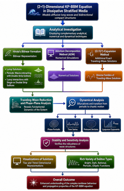
In this study, the (2+1)-dimensional Kadomtsev-Petviashvili-Benjamin-Bona-Mahony (KP-BBM) equation representing diffusive long waves and bidirectional compact structures in dissipative stratified media is investigated analytically. The bilinear representation, which immediately produces lump solutions, periodic waves interacting with double strip solitons, and lump interactions with single or double strip solitons, is provided by Hirota's bilinear formalism. In addition, we use the Adomian decomposition methodology for numerical simulations, and the $ (G'/G^{2}) $-expansion method provides additional accurate traveling-wave solutions. Phase-plane analysis and a traveling-wave reduction reveal the fundamental dynamics of the system. We use phase portraits, time series, Poincaré sections, and Lyapunov exponents to analyze bifurcations and the change from periodic to chaotic motion; further stability and sensitivity tests verify the robustness of the wave structures. The two- and three-dimensional visualizations of the solutions show that the model has a wide variety of soliton types, including bright, dark, rational, periodic, and elliptic functions. Overall, these results sharpen our understanding of the complex nonlinear behavior and propagation properties inherent in the KP-BBM equation.
Citation: Kalim U. Tariq, R. Nadir Tufail, Mohammed Ahmed Alomair. Soliton interactions, bifurcations, and chaos in the (2+1)-dimensional KP-BBM equation for diffusive long waves in stratified media[J]. AIMS Mathematics, 2026, 11(11): 38609-38652. doi: 10.3934/math.20261490
In this study, the (2+1)-dimensional Kadomtsev-Petviashvili-Benjamin-Bona-Mahony (KP-BBM) equation representing diffusive long waves and bidirectional compact structures in dissipative stratified media is investigated analytically. The bilinear representation, which immediately produces lump solutions, periodic waves interacting with double strip solitons, and lump interactions with single or double strip solitons, is provided by Hirota's bilinear formalism. In addition, we use the Adomian decomposition methodology for numerical simulations, and the $ (G'/G^{2}) $-expansion method provides additional accurate traveling-wave solutions. Phase-plane analysis and a traveling-wave reduction reveal the fundamental dynamics of the system. We use phase portraits, time series, Poincaré sections, and Lyapunov exponents to analyze bifurcations and the change from periodic to chaotic motion; further stability and sensitivity tests verify the robustness of the wave structures. The two- and three-dimensional visualizations of the solutions show that the model has a wide variety of soliton types, including bright, dark, rational, periodic, and elliptic functions. Overall, these results sharpen our understanding of the complex nonlinear behavior and propagation properties inherent in the KP-BBM equation.

| [1] |
F. Badshah, Ammara, S. Asghar, Ziauddin, S. H. Dong, Investigation of diffraction grating in three-level gain medium, Opt. Laser Technol., 177 (2024), 111104. https://doi.org/10.1016/j.optlastec.2024.111104 doi: 10.1016/j.optlastec.2024.111104
|
| [2] |
K. U. Tariq, M. Inc, A. Pashrashide, M. Zubair, L. Akinyemi, On the structure of unsteady Korteweg-de Vries model arising in shallow water, J. Ocean Eng. Sci., 2022, In press. https://doi.org/10.1016/j.joes.2022.01.011 |
| [3] |
F. Badshah, K. U. Tariq, A. Bekir, R. N. Tufail, H. Ilyas, Lump, periodic, travelling, semi-analytical solutions and stability analysis for the Ito integro-differential equation arising in shallow water waves, Chaos Solitons Fract., 182 (2024), 114783. https://doi.org/10.1016/j.chaos.2024.114783 doi: 10.1016/j.chaos.2024.114783
|
| [4] |
K. U. Tariq, A. Bekir, S. Nisar, The dynamical structures of the Sharma-Tasso-Olver model in doubly dispersive medium, Chaos Solitons Fract., 177 (2023), 114290. https://doi.org/10.1016/j.chaos.2023.114290 doi: 10.1016/j.chaos.2023.114290
|
| [5] |
A. R. Seadawy, A. Ali, A. Bekir, A. C. Cevikel, Ö. Guner, Novel exact wave solutions of the (4+1)-dimensional Boiti-Leon-Manna-Pempinelli model via application of three mathematical methods, Opt. Quantum Electron., 56 (2024), 1143. https://doi.org/10.1007/s11082-024-06997-1 doi: 10.1007/s11082-024-06997-1
|
| [6] |
S. T. R. Rizvi, S. Ahmed, Resonant collisions among X-type, multi-lump, generalized breathers, N-solitons and rogue waves in plasma, Optik, 292 (2023), 171390. https://doi.org/10.1016/j.ijleo.2023.171390 doi: 10.1016/j.ijleo.2023.171390
|
| [7] |
K. U. Tariq, A. R. Seadawy, S. T. R. Rizvi, R. Javed, Some optical soliton solutions to the generalized (1+1)-dimensional perturbed nonlinear Schrödinger equation using two analytical approaches, Int. J. Mod. Phys. B, 36 (2022), 2250177. https://doi.org/10.1142/S0217979222501776 doi: 10.1142/S0217979222501776
|
| [8] |
M. Inc, New solitary wave solutions with compact support and Jacobi elliptic function solutions for the nonlinearly dispersive Boussinesq equations, Chaos Solitons Fract., 37 (2008), 792–798. https://doi.org/10.1016/j.chaos.2006.09.064 doi: 10.1016/j.chaos.2006.09.064
|
| [9] |
F. Badshah, K. U. Tariq, A. Bekir, On the solitonic wave structures for the perturbed nonlinear Schrödinger equation arising in optical fibers, Opt. Quantum Electron., 56 (2024), 127. https://doi.org/10.1007/s11082-023-05625-8 doi: 10.1007/s11082-023-05625-8
|
| [10] |
D. Kumar, K. Hosseini, F. Samadani, The sine-Gordon expansion method to look for the traveling wave solutions of the Tzitzéica type equations in nonlinear optics, Optik, 149 (2017), 439–446. https://doi.org/10.1016/j.ijleo.2017.09.066 doi: 10.1016/j.ijleo.2017.09.066
|
| [11] |
T. Islam, A. Akbar, H. Rezazadeh, A. Bekir, New-fashioned solitons of coupled nonlinear Maccari systems describing the motion of solitary waves in fluid flow, J. Ocean Eng. Sci., 9 (2024), 353–363. https://doi.org/10.1016/j.joes.2022.03.003 doi: 10.1016/j.joes.2022.03.003
|
| [12] |
S. Carillo, M. L. Schiavo, C. Schiebold, Bäcklund transformations and non-abelian nonlinear evolution equations: a novel Bäcklund chart, SIGMA, 12 (2016), 087. https://doi.org/10.3842/SIGMA.2016.087 doi: 10.3842/SIGMA.2016.087
|
| [13] |
C. Q. Dai, Y. Y. Wang, Notes on the equivalence of different variable separation approaches for nonlinear evolution equations, Commun. Nonlinear Sci. Numer. Simul., 19 (2014), 19–28. https://doi.org/10.1016/j.cnsns.2013.05.027 doi: 10.1016/j.cnsns.2013.05.027
|
| [14] |
X. G. Geng, G. L. He, Some new integrable nonlinear evolution equations and Darboux transformation, J. Math. Phys., 51 (2010), 033514. https://doi.org/10.1063/1.3355192 doi: 10.1063/1.3355192
|
| [15] |
E. Misirli, Y. Gurefe, Exp-function method for solving nonlinear evolution equations, Math. Comput. Appl., 16 (2011), 258–266. https://doi.org/10.3390/mca16010258 doi: 10.3390/mca16010258
|
| [16] |
K. U. Tariq, A. M. Wazwaz, R. N. Tufail, Lump, periodic and travelling wave solutions to the (2+1)-dimensional pKP-BKP model, Eur. Phys. J. Plus, 137 (2022), 1–22. https://doi.org/10.1140/epjp/s13360-022-03301-6 doi: 10.1140/epjp/s13360-022-03301-6
|
| [17] |
Z. B. Yu, C. H. Zhu, J. S. Zhao, L. Zou, Inverse scattering transform of the general three-component nonlinear Schrödinger equation and its multisoliton solutions, Appl. Math. Lett., 128 (2022), 107874. https://doi.org/10.1016/j.aml.2021.107874 doi: 10.1016/j.aml.2021.107874
|
| [18] |
S. W. Yao, K. U. Tariq, M. Inc, R. N. Tufail, Modulation instability analysis and soliton solutions of the modified BBM model arising in dispersive medium, Results Phys., 46 (2023), 106274. https://doi.org/10.1016/j.rinp.2023.106274 doi: 10.1016/j.rinp.2023.106274
|
| [19] |
M. Mirzazadeh, A. Akbulut, F. Tascan, L. Akinyemi, A novel integration approach to study the perturbed Biswas-Milovic equation with Kudryashov's law of refractive index, Optik, 252 (2022), 168529. https://doi.org/10.1016/j.ijleo.2021.168529 doi: 10.1016/j.ijleo.2021.168529
|
| [20] |
M. A. Abdelkawy, A. H. Bhrawy, E. Zerrad, A. Biswas, Application of tanh method to complex coupled nonlinear evolution equations, Acta Phys. Polon. A, 129 (2016), 278–283. https://doi.org/10.12693/APhysPolA.129.278 doi: 10.12693/APhysPolA.129.278
|
| [21] |
R. C. López, G. H. Sun, O. Camacho-Nieto, C. Yáñez-Márquez, S. H. Dong, Analytical traveling-wave solutions to a generalized Gross-Pitaevskii equation with some new time and space varying nonlinearity coefficients and external fields, Phys. Lett. A, 381 (2017), 2978–2985. https://doi.org/10.1016/j.physleta.2017.07.012 doi: 10.1016/j.physleta.2017.07.012
|
| [22] |
X. L. Mai, W. Li, S. H. Dong, Exact solutions to the nonlinear Schrödinger equation with time-dependent coefficients, Adv. High Energy Phys., 2021 (2021), 6694980. https://doi.org/10.1155/2021/6694980 doi: 10.1155/2021/6694980
|
| [23] |
W. Li, C. F. Jiang, J. W. Huo, Y. S. Guo, Y. Shen, S. H. Dong, Gaussian solitary-wave solutions of a generalized logarithmic nonlinear Schrödinger equation with external potentials, Phys. Lett. A, 592 (2026), 131984. https://doi.org/10.1016/j.physleta.2026.131984 doi: 10.1016/j.physleta.2026.131984
|
| [24] |
W. X. Ma, Lump solutions to the Kadomtsev-Petviashvili equation, Phys. Lett. A, 379 (2015), 1975–1978. https://doi.org/10.1016/j.physleta.2015.06.061 doi: 10.1016/j.physleta.2015.06.061
|
| [25] |
A. M. Wazwaz, Exact solutions of compact and noncompact structures for the KP-BBM equation, Appl. Math. Comput., 169 (2005), 700–712. https://doi.org/10.1016/j.amc.2004.09.061 doi: 10.1016/j.amc.2004.09.061
|
| [26] |
A. M. Wazwaz, Two new integrable Kadomtsev-Petviashvili equations with time-dependent coefficients: multiple real and complex soliton solutions, Waves Random Complex Media, 30 (2020), 776–786. https://doi.org/10.1080/17455030.2018.1559962 doi: 10.1080/17455030.2018.1559962
|
| [27] |
A. R. Seadawy, Travelling-wave solutions of a weakly nonlinear two-dimensional higher-order Kadomtsev-Petviashvili dynamical equation for dispersive shallow-water waves, Eur. Phys. J. Plus, 132 (2017), 29. https://doi.org/10.1140/epjp/i2017-11313-4 doi: 10.1140/epjp/i2017-11313-4
|
| [28] |
M. A. Salam, M. A. Akbar, M. Z. Ali, M. Inc, The higher-order nonlinearity and parametric effects on dust-ion-acoustic shock waves, Phys. Scr., 97 (2022), 125605. https://doi.org/10.1088/1402-4896/ac9dc8 doi: 10.1088/1402-4896/ac9dc8
|
| [29] |
H. Rezazadeh, M. Inc, D. Baleanu, New solitary wave solutions for variants of (3+1)-dimensional Wazwaz-Benjamin-Bona-Mahony equations, Front. Phys., 8 (2020), 332. https://doi.org/10.3389/fphy.2020.00332 doi: 10.3389/fphy.2020.00332
|
| [30] |
A. M. Wazwaz, H. Triki, Soliton solutions for a generalized KdV and BBM equations with time-dependent coefficients, Commun. Nonlinear Sci. Numer. Simul., 16 (2011), 1122–1126. https://doi.org/10.1016/j.cnsns.2010.06.024 doi: 10.1016/j.cnsns.2010.06.024
|
| [31] |
A. M. Wazwaz, The extended tanh method for new compact and noncompact solutions for the KP-BBM and the ZK-BBM equations, Chaos Solitons Fract., 38 (2008), 1505–1516. https://doi.org/10.1016/j.chaos.2007.01.135 doi: 10.1016/j.chaos.2007.01.135
|
| [32] |
J. C. Saut, N. Tzvetkov, Global well-posedness for the KP-BBM equations, Appl. Math. Res. eXpress, 2004 (2004), 1–16. https://doi.org/10.1155/S1687120004010718 doi: 10.1155/S1687120004010718
|
| [33] |
M. N. Alam, M. A. Akbar, Exact traveling wave solutions of the KP-BBM equation by using the new approach of generalized (G'/G)-expansion method, SpringerPlus, 2 (2013), 617. https://doi.org/10.1186/2193-1801-2-617 doi: 10.1186/2193-1801-2-617
|
| [34] |
S. Q. Tang, X. L. Huang, W. T. Huang, Bifurcations of travelling wave solutions for the generalized KP-BBM equation, Appl. Math. Comput., 216 (2010), 2881–2890. https://doi.org/10.1016/j.amc.2010.03.139 doi: 10.1016/j.amc.2010.03.139
|
| [35] |
J. Q. Lü, S. Bilige, X. Q. Gao, Y. X. Bai, R. F. Zhang, Abundant lump solutions and interaction phenomena to the Kadomtsev-Petviashvili-Benjamin-Bona-Mahony equation, J. Appl. Math. Phys., 6 (2018), 1733–1747. https://doi.org/10.4236/jamp.2018.68148 doi: 10.4236/jamp.2018.68148
|
| [36] |
J. Tan, Z. H. Deng, T. L. Wu, B. Tang, Propagation and interaction of magnetic solitons in a ferromagnetic thin film with the interfacial Dzyaloshinskii-Moriya interaction, J. Magn. Magn. Mater., 475 (2019), 445–452. https://doi.org/10.1016/j.jmmm.2018.11.048 doi: 10.1016/j.jmmm.2018.11.048
|
| [37] |
Z. H. Deng, T. L. Wu, B. Tang, X. Y. Wang, H. P. Zhao, K. Deng, Breathers and rogue waves in a ferromagnetic thin film with the Dzyaloshinskii-Moriya interaction, Eur. Phys. J. Plus, 133 (2018), 450. https://doi.org/10.1140/epjp/i2018-12311-8 doi: 10.1140/epjp/i2018-12311-8
|
| [38] |
Z. H. Deng, X. Chang, J. N. Tan, B. Tang, K. Deng, Characteristics of the lumps and stripe solitons with interaction phenomena in the (2+1)-dimensional Caudrey-Dodd-Gibbon-Kotera-Sawada equation, Int. J. Theor. Phys., 58 (2019), 92–102. https://doi.org/10.1007/s10773-018-3912-2 doi: 10.1007/s10773-018-3912-2
|
| [39] |
S. F. Tian, Lie symmetry analysis, conservation laws and solitary wave solutions to a fourth-order nonlinear generalized Boussinesq water wave equation, Appl. Math. Lett., 100 (2020), 106056. https://doi.org/10.1016/j.aml.2019.106056 doi: 10.1016/j.aml.2019.106056
|
| [40] |
H. Wang, S. F. Tian, T. T. Zhang, Y. Chen, Y. Fang, General lump solutions, lumpoff solutions, and rogue wave solutions with predictability for the (2+1)-dimensional Korteweg-de Vries equation, Comput. Appl. Math., 38 (2019), 164. https://doi.org/10.1007/s40314-019-0938-x doi: 10.1007/s40314-019-0938-x
|
| [41] |
W. Q. Peng, S. F. Tian, X. B. Wang, T. T. Zhang, Y. Fang, Riemann-Hilbert method and multi-soliton solutions for three-component coupled nonlinear Schrödinger equations, J. Geom. Phys., 146 (2019), 103508. https://doi.org/10.1016/j.geomphys.2019.103508 doi: 10.1016/j.geomphys.2019.103508
|
| [42] |
W. Q. Peng, S. F. Tian, X. B. Wang, T. T. Zhang, Characteristics of rogue waves on a periodic background for the Hirota equation, Wave Motion, 93 (2020), 102454. https://doi.org/10.1016/j.wavemoti.2019.102454 doi: 10.1016/j.wavemoti.2019.102454
|
| [43] |
D. Guo, S. F. Tian, X. B. Wang, T. T. Zhang, Dynamics of lump solutions, rogue wave solutions and traveling wave solutions for a (3+1)-dimensional VC-BKP equation, East Asian J. Appl. Math., 9 (2019), 780–796. https://doi.org/10.4208/eajam.310319.040619 doi: 10.4208/eajam.310319.040619
|
| [44] |
W. Q. Peng, S. F. Tian, T. T. Zhang, Dynamics of the soliton waves, breather waves, and rogue waves to the cylindrical Kadomtsev-Petviashvili equation in pair-ion-electron plasma, Phys. Fluids, 31 (2019), 102107. https://doi.org/10.1063/1.5116231 doi: 10.1063/1.5116231
|
| [45] |
W. Q. Peng, S. F. Tian, T. T. Zhang, Dynamics of breather waves and higher-order rogue waves in a coupled nonlinear Schrödinger equation, Europhys. Lett., 123 (2018), 50005. https://doi.org/10.1209/0295-5075/123/50005 doi: 10.1209/0295-5075/123/50005
|
| [46] |
R. Hirota, Exact solution of the Korteweg-de Vries equation for multiple collisions of solitons, Phys. Rev. Lett., 27 (1971), 1192. https://doi.org/10.1103/PhysRevLett.27.1192 doi: 10.1103/PhysRevLett.27.1192
|
| [47] |
W. X. Ma, Y. Zhou, Lump solutions to nonlinear partial differential equations via Hirota bilinear forms, J. Differ. Equ., 264 (2018), 2633–2659. https://doi.org/10.1016/j.jde.2017.10.033 doi: 10.1016/j.jde.2017.10.033
|
| [48] |
R. Hirota, The direct method in soliton theory, Cambridge University Press, 2004. https://doi.org/10.1017/CBO9780511543043 |
| [49] |
A. Wolf, J. B. Swift, H. L. Swinney, J. A. Vastano, Determining Lyapunov exponents from a time series, Phys. D, 16 (1985), 285–317. https://doi.org/10.1016/0167-2789(85)90011-9 doi: 10.1016/0167-2789(85)90011-9
|
Figures(23) / Tables(4)

Kalim U. Tariq, R. Nadir Tufail, Mohammed Ahmed Alomair. Soliton interactions, bifurcations, and chaos in the (2+1)-dimensional KP-BBM equation for diffusive long waves in stratified media[J]. AIMS Mathematics, 2026, 11(11): 38609-38652. doi: 10.3934/math.20261490

Schematic workflow for analyzing the $ (2+1) $-dimensional KP-BBM equation
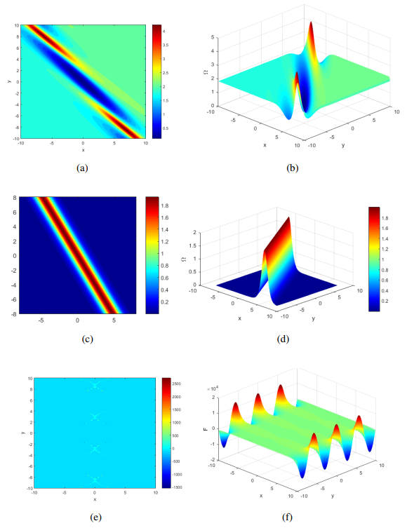
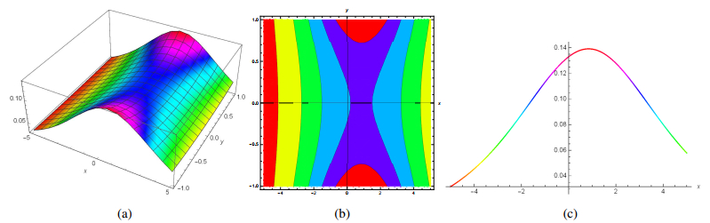
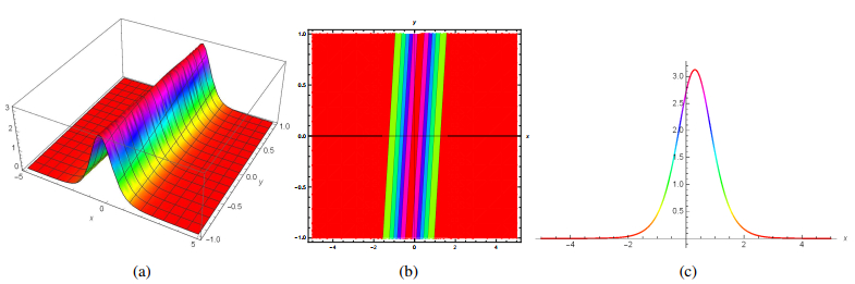
Visualization of periodic soliton $ \Omega_{2}(x, y, t) $, strip-like soliton $ \Omega_{4}(x, y, t) $, and interaction of a lump wave with double-stripe soliton $ \Omega_{8}(x, y, t) $
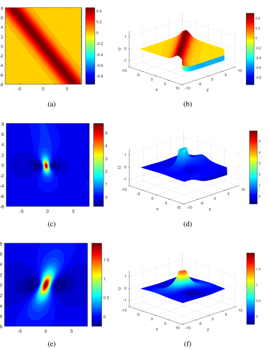
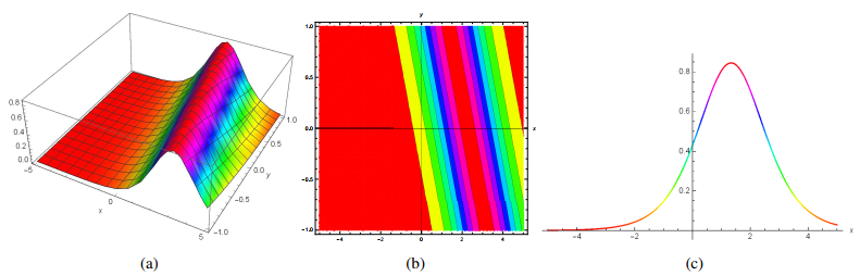
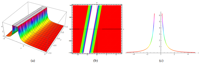
Visualization of strip soliton $ \Omega_{12}(x, y, t) $, interaction of a lump with periodic waves $ \Omega_{14}(x, y, t) $, and interaction of lump and periodic wave with a double-stripe soliton $ \Omega_{15}(x, y, t) $
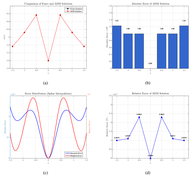
The ADM numerical approximation and the exact solution are compared. The exact and ADM solutions are shown in panel (a); the two curves are almost identical. The absolute error is displayed as a bar chart in panel (b). The error distribution produced by spline interpolation is shown in panel (c). The relative error of the ADM solution is shown in panel (d)
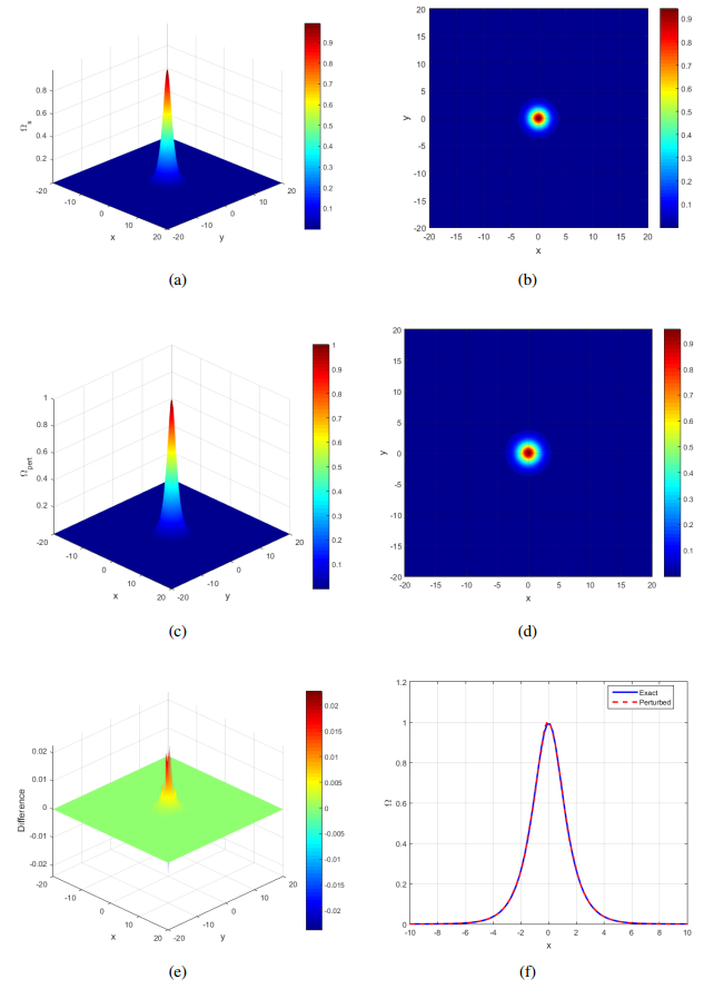
Stability characterization of the solitary wave under small perturbations: (a) the exact solitary wave in 3D, a smooth and symmetric peak; (b) its 2D contour plot, displaying nested closed loops; (c) the same wave after adding a small perturbation to the initial condition, shown in 3D; the shape now displays ripples or drift; (d) the contour plot of the perturbed wave, revealing distorted loops and broken symmetry; (e) the difference $ \Omega_{\text{pert}} - \Omega_{\text{exact}} $ across the domain, indicating where the perturbation has the biggest effect; and (f) a cross-section at $ y = 0 $
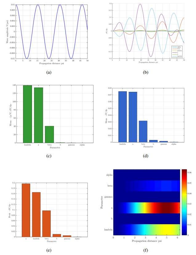
Sensitivity analysis of the wave solution in two dimensions: (a) The baseline wave profile under the original, unperturbed parameter set; (b) sensitivity traces plotted for each parameter one at a time, illustrating how the wave shape changes when a single parameter is increased or decreased; (c) mean relative sensitivity, which averages the response across the entire domain to identify the most influential parameters overall; (d) time-averaged sensitivities, which filter out rapid oscillations to reveal slow, persistent parameter effects; (e) maximum sensitivity recorded anywhere in the domain, indicating the parameter that causes the strongest local reaction; and (f) a heatmap covering a two-parameter grid, where bright patches indicate stable regions
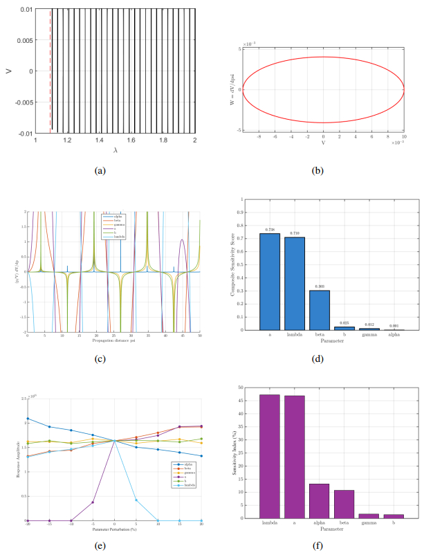
Sensitivity and bifurcation analysis using the one-parameter-at-a-time (OAT) method: (a) A two-dimensional bifurcation diagram depicting stability loss and regime changes when two parameters reach critical thresholds. (b) Phase portraits that depict qualitative changes in the flow, such as the formation of limit cycles or separatrices. (c) Relative sensitivity profiles show the percent change in the solution per one-percent parameter modification. (d) A bar chart ranking parameters according to their mean or peak sensitivity. (e) OAT response curves: wave behavior when each parameter is varied independently. (f) Ranking of OAT sensitivity characteristics based on average or greatest variation from (e)
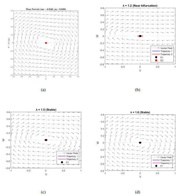
Phase portraits at four corresponding parameter settings show how sustained oscillations give way to steady decay: (a) The trajectory traces a clean, repeating loop at $ \mu = 0.5640 $ and $ \nu = 0.0444 $, indicating a stable limit cycle; (b) the loop warps and no longer closes neatly near the tipping point $ \lambda = 1.2 $, indicating that the system is approaching a bifurcation; and (c) the cycle has collapsed into a stable focus at $ \lambda = 1.5 $. Instead of spiraling continually, the trajectory spirals inward to a single point; and (d) the stronger value $ \lambda = 1.8 $
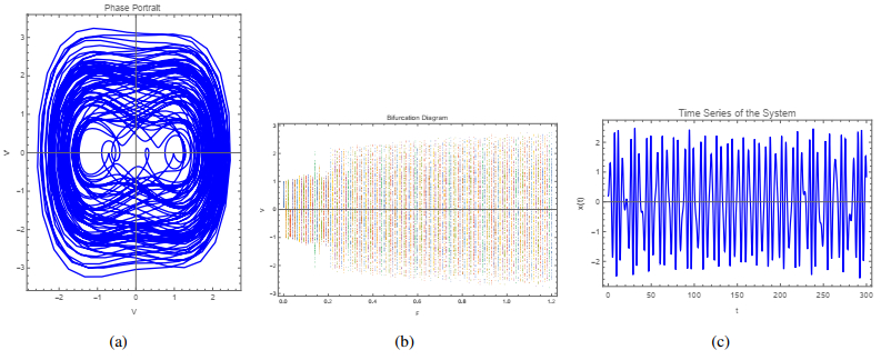
(a) Phase characterizations demonstrate how system properties impact trajectories in the $ (x, y) $-plane. Closed periodic orbits are replaced by complex aperiodic formations, which indicate the emergence of chaos and nonlinearities. (b) $ x $ bifurcation diagram with respect to the control variable. Point density and splitting show regime limits, while a pitchfork bifurcation initiates period-doubling sequences that result in chaos. (c) Time series $ x(\xi) $ for chosen parameters. Periodic motion is shown by repeated oscillations, but chaotic behavior and sensitivity to initial conditions are revealed by irregular fluctuations. Together, the panels depict the change from order to chaos when parameters change
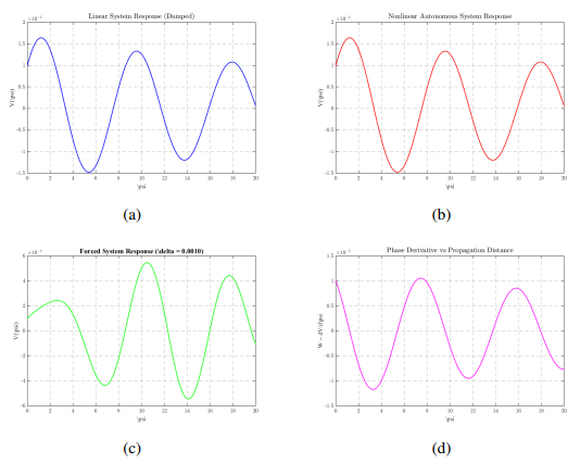
Time-domain behavior in four dynamical scenarios: (a) A damped linear response, in which the amplitude begins at a certain initial value and then smoothly decreases toward zero without ever rebounding or oscillating on its own; (b) an autonomous nonlinear system, in which $ V(\psi) $ and $ W(\psi) $ start at $ 0.040 $ before falling to a repeating two-step pattern of $ 0.020 $ and $ 0.025 $; (c) the identical nonlinear system with a tiny forcing amplitude $ \delta = 0.010 $ added; this alternate cycle continuous indefinitely without any outside input. The phase derivative $ d\psi/dt $ from the alternating $ V/W $ sequence; (d) long-term attractor. Both are almost identical to the unforced example, demonstrating that weak forcing has no substantial effect on the underlying oscillation. The derivative's sign alternates periodically, indicating a phase quadrature relation in which $ V $ and $ W $ are a quarter-step out of phase
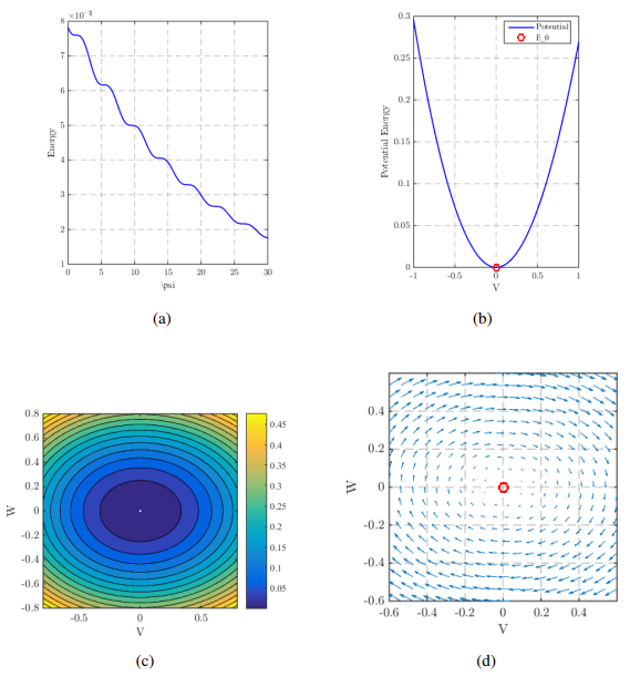
Dynamical analysis: (a) Energy diminishes uniformly with damping and approaches zero. (b) Energy potential landscape: the system behaves like a ball rolling along a curve; the deepest wells represent the most stable equilibria. (c) Phase portrait with energy contours: nested ovals indicate confined motion, whereas open curves imply unbounded motion. (d) Local phase portraits: a steady spiral at a potential minimum, and a saddle with two incoming and outgoing separatrices
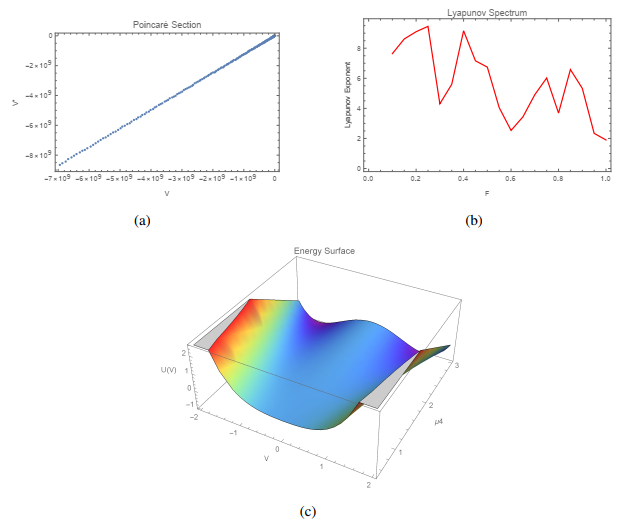
(a) The Poincaré section of the system as found by stroboscopic sampling at $ \xi_n = 2\pi n/\omega $. The unique points reveal the phase space structure of the system. A fractal-like distribution confirms chaotic dynamics, while a limited number of points represents periodic behavior. (b) Variations in the control parameter's largest Lyapunov exponent. Positive values of the exponent confirm the presence of chaotic dynamics, while negative values show stable periodic motion. The transition point indicates the onset of chaos in the system. (c) Energy surface (Hamiltonian landscape) of the dynamical system illustrating the variation of total energy $ E(x, y) $ in the phase space. The topology of the energy landscape clearly shows a transition from a single-well structure to a double-well potential as the control parameter $ \mu_4 $ crosses the critical value $ \mu_1 $, indicating bistability and phase space restructuring associated with bifurcation behavior
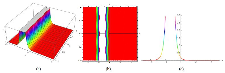
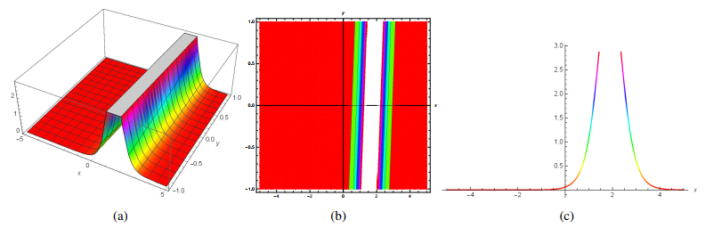
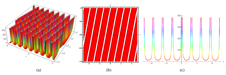
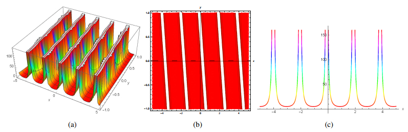
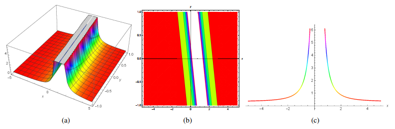
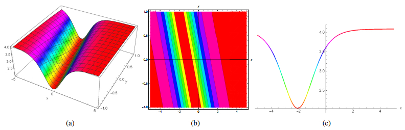
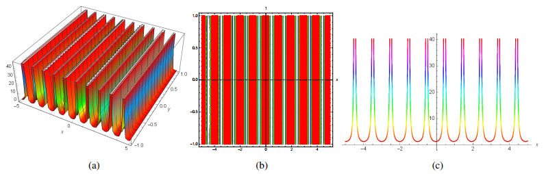
Portraits of the solution $ |\Omega_2(x, y, t)| $ considering $ \alpha _0 = -0.6 $, $ \alpha _1 = 0.25 $, $ \alpha _3 = 0.5 $, $ \gamma = 0.3, \; \alpha = 0.1, \; \xi _0 = 0.2, \; \xi _2 = 0.4, \; \xi _1 = 0.5, \text{and}\; \beta = 0.2 $
Portraits of the solution $ |\Omega_3(x, y, t)| $ considering $ \gamma _0 = 0.3 $, $ \gamma _1 = -2.5 $, $ \alpha = 0.5 $, $ \gamma _2 = 0.75 $, $ \xi _0 = 0.8, \; \gamma = 0.7, \; \xi _3 = 0.16, \text{and}\; \beta = 0.6 $
Portraits of the solution $ |\Omega_7(x, y, t)| $ considering $ \beta = 0.3 $, $ \gamma _0 = 0.5 $, $ \gamma _1 = 0.65 $, $ \alpha = 0.5 $, $ \gamma _2 = 0.6, \text{and}\; \gamma = 0.4 $
Portraits of the solution $ |\Omega_5(x, y, t)| $ considering $ \alpha _0 = 0.25 $, $ \alpha _1 = 1.2 $, $ \alpha _2 = -1.1 $, $ \beta _0 = 0.1 $, $ \alpha = 0.5, \; \beta _1 = 1.1, \; \beta _2 = -1.2, \; \beta = 0.6, \; \beta _3 = 0.5, \; \xi _1 = 0.25, \text{and}\; \gamma = -0.7 $
Portraits of the solution $ |\Omega_{10}(x, y, t)| $ considering $ \beta = 0.3 $, $ \gamma _0 = 1.55 $, $ \gamma _1 = 1.75 $, $ \alpha = 0.5 $, $ \gamma _3 = 0.9, \text{and}\; \gamma = 0.4 $
Portraits of the solution $ |\Omega_{16}(x, y, t)| $ considering $ \beta _0 = 0.55 $, $ \beta _1 = -1.5 $, $ \beta _2 = 0.255 $, $ \alpha = 2.1 $, $ \gamma _0 = 0.25 $, $ \xi _2 = 2.5 $, $ \beta = 0.2, \; \xi _3 = 0.45, \text{and}\; \gamma = 0.5 $
Portraits of the solution $ |\Omega_{11}(x, y, t)| $ considering $ \beta = 0.35 $, $ \gamma _0 = 0.2 $, $ \gamma _1 = 2.5 $, $ \alpha = 0.25 $, $ \gamma _2 = -2.3, \text{and}\; \gamma = 0.45 $
Portraits of the solution $ |\Omega_{13}(x, y, t)| $ considering $ \beta = 0.2 $, $ \gamma _0 = 0.1 $, $ \gamma _1 = 1.6 $, $ \alpha = 0.1 $, $ \gamma _3 = 1.1, \text{and}\; \gamma = 0.3 $
Portraits of the solution $ |\Omega_{18}(x, y, t)| $ considering $ a = -0.2 $, $ \kappa = -1.5 $, $ \omega = -1.6 $, $ \alpha = 0.25 $, $ \chi_1 = 1, \; \beta = -0.15, \; \chi_2 = 1.2, \; \gamma = 0.3, \text{and}\; b = -0.1 $
Portraits of the solution $ |\Omega_{21}(x, y, t)| $ considering $ a = 1.2 $, $ \kappa = -0.5 $, $ \alpha = 1.25 $, $ \omega = -0.6 $, $ \beta = 1.5 $, $ \chi_1 = 1.2, \; b = 1.1, \; \chi_2 = 1.5, \text{and}\; \gamma = 1.3 $
Portraits of the solution $ |\Omega_{23}(x, y, t)| $ considering $ \kappa = 1.1 $, $ \omega = 1.6 $, $ \chi_1 = 1.5 $, $ \chi_2 = 1.2 $, $ a = 1.2 $, $ b = 1.1 $, $ \alpha = 1.25, \; \beta = 1.15, \text{and}\; \gamma = 1.3 $




 DownLoad: