The Schrödinger equation has an important place among the partial differential equations used in quantum mechanics, since it describes the time evolution of a physical system. In this paper, a numerical method is developed for the time-fractional nonlinear Schrödinger equation involving the Caputo fractional derivative. The temporal discretization is constructed using the L1 formula together with Crank–Nicolson-type averaging, and the nonlinear coefficient is evaluated explicitly at the previous time level. For the spatial discretization, a collocation method based on cubic B-splines is combined with a high-order approximation of the second spatial derivative. The resulting formulation leads to a linear algebraic system at each time step for the coefficients associated with the real and imaginary parts of the solution. A local consistency analysis is presented for sufficiently smooth solutions. The analysis shows that the complete discretization has local truncation error of order $ O(\Delta t+h^4) $ so that the temporal discretization is first-order consistent, whereas the high-order spatial approximation is fourth-order accurate. These behaviors are also examined separately through temporal and spatial refinement studies. A nonsmooth test problem with a weak initial singularity is also considered to examine the numerical behavior of the method for a solution with limited temporal regularity. The numerical results exhibit approximately first-order temporal convergence for the smooth test problems and approximately fourth-order spatial convergence for Problem 1. Numerical experiments are further used to compare the performance of cubic, trigonometric, and uniform hyperbolic polynomial B-spline bases. A Fourier analysis of the corresponding linearized frozen-coefficient recurrence is also discussed. The numerical results and comparisons illustrate the accuracy of the proposed high-order B-spline collocation approach for the considered time-fractional Schrödinger problems.
Citation: Alaattin Esen, Murat Önal, Berat Karaagac. Enhancing accuracy in time-fractional Schrödinger equation: a high-order B-spline collocation approach[J]. AIMS Mathematics, 2026, 11(11): 37837-37878. doi: 10.3934/math.20261463
The Schrödinger equation has an important place among the partial differential equations used in quantum mechanics, since it describes the time evolution of a physical system. In this paper, a numerical method is developed for the time-fractional nonlinear Schrödinger equation involving the Caputo fractional derivative. The temporal discretization is constructed using the L1 formula together with Crank–Nicolson-type averaging, and the nonlinear coefficient is evaluated explicitly at the previous time level. For the spatial discretization, a collocation method based on cubic B-splines is combined with a high-order approximation of the second spatial derivative. The resulting formulation leads to a linear algebraic system at each time step for the coefficients associated with the real and imaginary parts of the solution. A local consistency analysis is presented for sufficiently smooth solutions. The analysis shows that the complete discretization has local truncation error of order $ O(\Delta t+h^4) $ so that the temporal discretization is first-order consistent, whereas the high-order spatial approximation is fourth-order accurate. These behaviors are also examined separately through temporal and spatial refinement studies. A nonsmooth test problem with a weak initial singularity is also considered to examine the numerical behavior of the method for a solution with limited temporal regularity. The numerical results exhibit approximately first-order temporal convergence for the smooth test problems and approximately fourth-order spatial convergence for Problem 1. Numerical experiments are further used to compare the performance of cubic, trigonometric, and uniform hyperbolic polynomial B-spline bases. A Fourier analysis of the corresponding linearized frozen-coefficient recurrence is also discussed. The numerical results and comparisons illustrate the accuracy of the proposed high-order B-spline collocation approach for the considered time-fractional Schrödinger problems.

| [1] |
B. N. Narahari Achar, B. T. Yale, J. W. Hanneken, Time fractional Schrödinger equation revisited, Adv. Math. Phys., 2013 (2013), 290216. https://doi.org/10.1155/2013/290216 doi: 10.1155/2013/290216
|
| [2] |
C. Sulem, P. L. Sulem, The nonlinear Schrödinger equation: self-focusing and wave collapse, Applied Mathematical Sciences, Vol. 139, New York: Springer, 1999. https://doi.org/10.1007/b98958 |
| [3] |
A. Amer, E. K. Jaradat, H. U. Rehman, Y. Yildirim, S. Abu Alrub, M. S. Ateto, Exact and numerical optical soliton solutions of the fractional quadratic–cubic nonlinear Schrödinger equation in conformable derivative framework, Sci. Rep., 16 (2026), 15118. https://doi.org/10.1038/s41598-026-43272-7 doi: 10.1038/s41598-026-43272-7
|
| [4] |
M. A. Mustafa, M. A. S. Murad, Soliton solutions for time-fractional (3+1)-dimensional nonlinear Schrödinger equation with cubic-quintic nonlinearity terms, Int. J. Comput. Math., 102 (2025), 1428–1442. https://doi.org/10.1080/00207160.2025.2499879 doi: 10.1080/00207160.2025.2499879
|
| [5] |
S. Panwar, R. M. Pandey, P. Rai, An analysis of the nonlinear time-fractional Schrödinger and coupled Klein–Gordon–Schrödinger equations, New Math. Nat. Comput., 2026, 1–21. https://doi.org/10.1142/S1793005728500172 |
| [6] |
A. Hagag, Z. Alqahtani, A. Arafa, Efficient analytic technique for fractional fourth-order cubic nonlinear Schrödinger equation, Rev. Int. Métodos Numér. Cálc. Diseño Ing., 41 (2025), 16. https://doi.org/10.23967/j.rimni.2024.10.60138 doi: 10.23967/j.rimni.2024.10.60138
|
| [7] |
A. A. M. Arafa, A. M. S. Hagag, Q-homotopy analysis transform method applied to fractional Kundu–Eckhaus equation and fractional massive Thirring model arising in quantum field theory, Asian-Eur. J. Math., 12 (2019), 1950045. https://doi.org/10.1142/S1793557119500451 doi: 10.1142/S1793557119500451
|
| [8] |
D. Shi, Z. Li, Neural network-driven exact solutions for the conformal nonlinear fractional Kolmogorov–Petrovskii–Piskunov model, Phys. Lett. A, 593 (2026), 132023. https://doi.org/10.1016/j.physleta.2026.132023 doi: 10.1016/j.physleta.2026.132023
|
| [9] |
H. Lv, Exact traveling wave solutions of the paraxial wave equation with conformable fractional derivative using an enhanced direct algebraic method, Symmetry, 18 (2026), 1300. https://doi.org/10.3390/sym18081300 doi: 10.3390/sym18081300
|
| [10] |
A. Mohebbi, M. Abbaszadeh, M. Dehghan, The use of a meshless technique based on collocation and radial basis functions for solving the time fractional nonlinear Schrödinger equation arising in quantum mechanics, Eng. Anal. Boundary Elem., 37 (2013), 475–485. https://doi.org/10.1016/j.enganabound.2012.12.002 doi: 10.1016/j.enganabound.2012.12.002
|
| [11] |
A. R. Hadhoud, A. A. M. Rageh, T. Radwan, Computational solution of the time-fractional Schrödinger equation by using trigonometric B-spline collocation method, Fractal Fract., 6 (2022), 127. https://doi.org/10.3390/fractalfract6030127 doi: 10.3390/fractalfract6030127
|
| [12] |
M. A. Bayrak, A. Demir, Numerical solution of space fractional Schrödinger equation by fractional Clique collocation method, Kafkas Üniv. Fen Bilimleri Enst. Derg., 18 (2025), 54–59. https://doi.org/10.58688/kujs.1702711 |
| [13] |
S. Nemati, S. Sedaghat, S. Arefi, A new numerical approach for solving space–time fractional Schrödinger differential equations via fractional-order Chelyshkov functions, Results Appl. Math., 26 (2025), 100584. https://doi.org/10.1016/j.rinam.2025.100584 doi: 10.1016/j.rinam.2025.100584
|
| [14] |
Y. Wang, B. Yin, Y. Liu, H. Li, Modified L1 Crank–Nicolson finite element methods with unconditional convergence for nonlinear time-fractional Schrödinger equations, Commun. Nonlinear Sci. Numer. Simul., 143 (2025), 108623. https://doi.org/10.1016/j.cnsns.2025.108623 doi: 10.1016/j.cnsns.2025.108623
|
| [15] |
X. Zhou, M. Zhang, C. Liao, Unconditionally stable L1-2 FEMs for nonlinear Schrödinger equations with the variable-order time-fractional derivative, Mathematics, 14 (2026), 1656. https://doi.org/10.3390/math14101656 doi: 10.3390/math14101656
|
| [16] |
M. Serik, R. Eskar, P. Huang, Numerical solution of time-fractional Schrödinger equation by using FDM, Axioms, 12 (2023), 816. https://doi.org/10.3390/axioms12090816 doi: 10.3390/axioms12090816
|
| [17] |
A. M. Hayat, M. Abbas, H. Emadifar, A. S. M. Alzaidi, T. Nazir, F. A. Abdullah, An efficient computational scheme for solving coupled time-fractional Schrödinger equation via cubic B-spline functions, PLoS ONE, 19 (2024), e0296909. https://doi.org/10.1371/journal.pone.0296909 doi: 10.1371/journal.pone.0296909
|
| [18] |
M. Önal, B. Karaağaç, A. Esen, An efficient higher-order trigonometric cubic B-spline collocation method for time-fractional Burgers equations, Int. J. Math. Comput. Eng., 4 (2026), 211–234. https://doi.org/10.2478/ijmce-2026-0013 doi: 10.2478/ijmce-2026-0013
|
| [19] |
C. Li, W. Deng, Remarks on fractional derivatives, Appl. Math. Comput., 187 (2007), 777–784. https://doi.org/10.1016/j.amc.2006.08.163 doi: 10.1016/j.amc.2006.08.163
|
| [20] |
Y. Lin, C. Xu, Finite difference/spectral approximations for the time-fractional diffusion equation, J. Comput. Phys., 225 (2007), 1533–1552. https://doi.org/10.1016/j.jcp.2007.02.001 doi: 10.1016/j.jcp.2007.02.001
|
| [21] |
H. Zhang, F. Liu, M. S. Phanikumar, M. M. Meerschaert, A novel numerical method for the time variable fractional order mobile–immobile advection–dispersion model, Comput. Math. Appl., 66 (2013), 693–701. https://doi.org/10.1016/j.camwa.2013.01.031 doi: 10.1016/j.camwa.2013.01.031
|
| [22] |
A. R. Khlefha, A comprehensive review of applications of spline function, Int. Acad. J. Sci. Eng., 11 (2024), 322–331. https://doi.org/10.9756/iajse/v11i1/iajse1138 doi: 10.9756/iajse/v11i1/iajse1138
|
| [23] |
V. Dahiya, Exploring B-spline functions for numerical solution of mathematical problems, Int. J. Multidiscip. Res. Dev., 2 (2015), 452–458. |
| [24] |
G. Walz, Identities for trigonometric B-splines with an application to curve design, BIT Numer. Math., 37 (1997), 189–201. https://doi.org/10.1007/BF02510180 doi: 10.1007/BF02510180
|
| [25] |
M. S. Palav, V. H. Pradhan, Redefined fourth order uniform hyperbolic polynomial B-splines based collocation method for solving advection–diffusion equation, Appl. Math. Comput., 484 (2025), 128992. https://doi.org/10.1016/j.amc.2024.128992 doi: 10.1016/j.amc.2024.128992
|
| [26] |
T. R. Lucas, Error bounds for interpolating cubic splines under various end conditions, SIAM J. Numer. Anal., 11 (1974), 569–584. https://doi.org/10.1137/0711049 doi: 10.1137/0711049
|
| [27] |
R. C. Mittal, R. Rohila, A fourth order cubic B-spline collocation method for the numerical study of the RLW and MRLW equations, Wave Motion, 80 (2018), 47–68. https://doi.org/10.1016/j.wavemoti.2018.04.001 doi: 10.1016/j.wavemoti.2018.04.001
|
| [28] |
R. Rohila, R. C. Mittal, Numerical study of reaction diffusion Fisher's equation by fourth order cubic B-spline collocation method, Math. Sci., 12 (2018), 79–89. https://doi.org/10.1007/s40096-018-0247-3 doi: 10.1007/s40096-018-0247-3
|
| [29] |
O. Taşbozan, Kesirli mertebeden kısmi diferansiyel denklemlerin B-spline sonlu eleman yöntemleri ile Çözümleri [Solutions of fractional order partial differential equations by B-spline finite element methods], PhD thesis, Turkey: İnönü University, 2015. |
Figures(8) / Tables(21)

Alaattin Esen, Murat Önal, Berat Karaagac. Enhancing accuracy in time-fractional Schrödinger equation: a high-order B-spline collocation approach[J]. AIMS Mathematics, 2026, 11(11): 37837-37878. doi: 10.3934/math.20261463

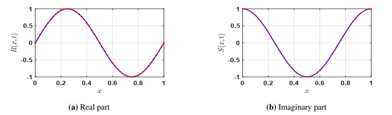
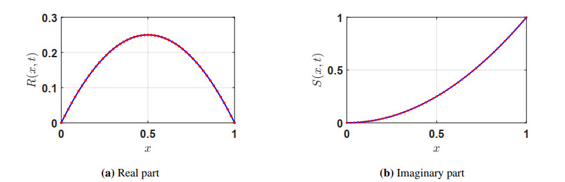
Comparison of the numerical solution (circles) and the exact solution (solid line) for the real and imaginary parts of Problem 1 for $ N = 50 $, $ \Delta t = 0.001 $, and $ \gamma = 0.5 $ at $ t_f = 1 $
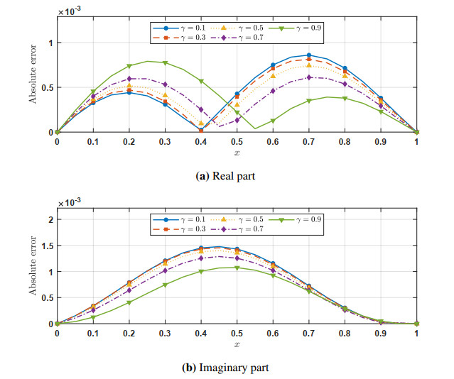
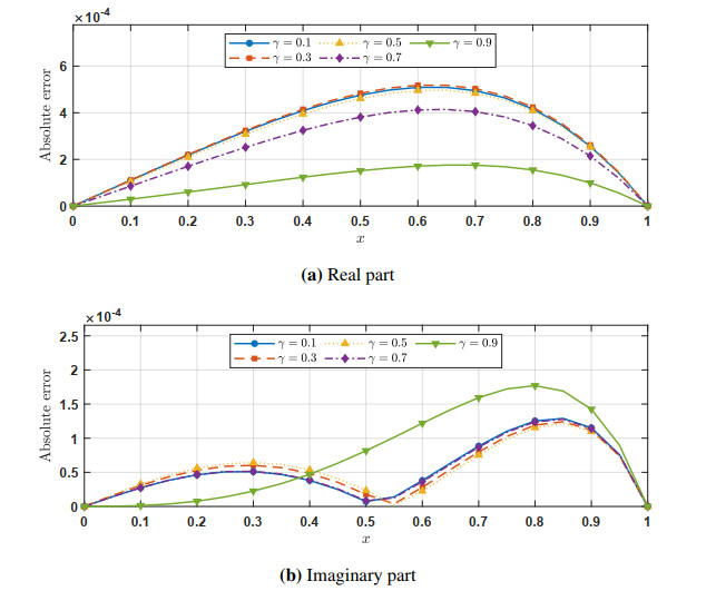
Distribution of the absolute error at $ t = 1 $ for the real part (top) and the imaginary part (bottom) of Problem 1 for $ N = 20 $; $ \Delta t = 0.01 $; and $ \gamma = 0.1, 0.3, 0.5, 0.7, 0.9 $
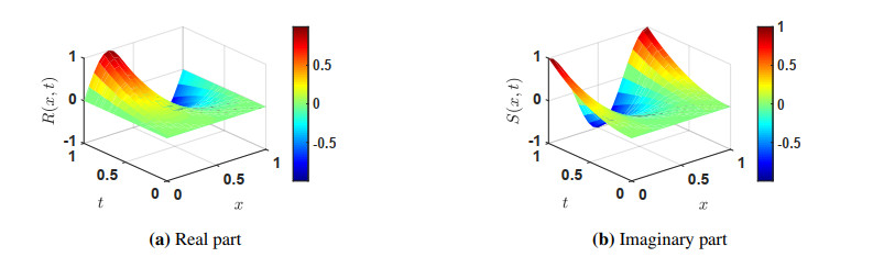
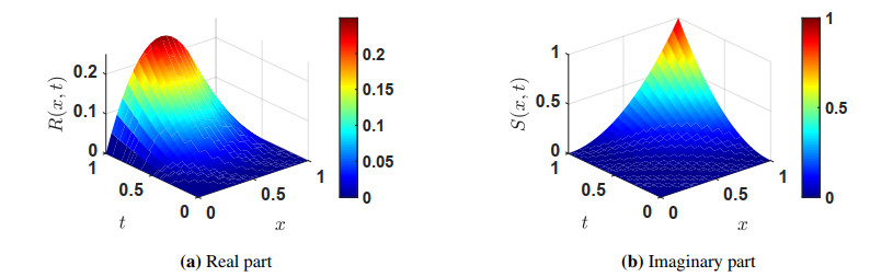
Space–time surfaces of the numerical solution for the real part (left) and the imaginary part (right) of Problem 1 for $ N = 20 $, $ \Delta t = 0.01 $, and $ \gamma = 0.5 $
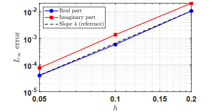
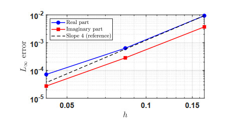
$ L_{\infty} $ error versus mesh size $ h $ for the real and imaginary parts of Problem 1 for $ \gamma = 0.5 $ and $ \Delta t = 0.00005 $. The dashed reference line has slope four
Comparison of the numerical solution (circles) and the exact solution (solid line) for the real and imaginary parts of Problem 2 for $ N = 50 $, $ \Delta t = 0.001 $, and $ \gamma = 0.5 $ at $ t_f = 1 $
Distribution of the absolute error across the domain at $ t = 1 $ for the real part (top) and the imaginary part (bottom) of Problem 2 for $ N = 20 $; $ \Delta t = 0.01 $; and $ \gamma = 0.1, 0.3, 0.5, 0.7, 0.9 $
Space–time surfaces of the numerical solution for the real part (left) and the imaginary part (right) of Problem 2 for $ N = 20 $, $ \Delta t = 0.01 $, and $ \gamma = 0.5 $
$ L_{\infty} $ error under a joint spatial–temporal refinement for the real and imaginary parts of Problem 2 at $ \gamma = 0.8 $, with $ \Delta t\propto h^{\log_2(10)}\approx h^{3.322} $; this refinement relation differs from the balanced relation $ \Delta t = Ch^4 $ used in Table \ref{tab:18}. The dashed reference line has slope four




 DownLoad: