We study a class of time-dependent mixed generalized Volterra–Fredholm integral equations with hypergeometric Banach space spatial kernel $X = C([0, T]; L^2(-1, 1))$. The formulation proposed involves several important singular kernels; as special cases, consider the logarithmic, Carleman, and complete elliptic kernels. The Banach fixed-point theorem is used to establish adequate conditions for existence and uniqueness under appropriate assumptions on the spatial kernel and the temporal memory function, with the contraction constraint $BM_G < \mu$. A quadrature-based Nyström-type discretization is employed for the numerical treatment of the spatial integral operator. Numerical studies are performed for the logarithmic, Carleman, complete elliptic, and general hypergeometric cases at selected times to investigate the effects of temporal memory, kernel singularity, and the kernel parameters on the computed solution. The numerical accuracy and convergence behavior are also examined through appropriate error and refinement measures.
Citation: Jihan Alahmadi, M. A. Abdou, M. Mahmoud Ismail. Analytical and numerical analysis of a time-dependent mixed integral equation with a hypergeometric kernel[J]. AIMS Mathematics, 2026, 11(11): 37764-37794. doi: 10.3934/math.20261460
We study a class of time-dependent mixed generalized Volterra–Fredholm integral equations with hypergeometric Banach space spatial kernel $X = C([0, T]; L^2(-1, 1))$. The formulation proposed involves several important singular kernels; as special cases, consider the logarithmic, Carleman, and complete elliptic kernels. The Banach fixed-point theorem is used to establish adequate conditions for existence and uniqueness under appropriate assumptions on the spatial kernel and the temporal memory function, with the contraction constraint $BM_G < \mu$. A quadrature-based Nyström-type discretization is employed for the numerical treatment of the spatial integral operator. Numerical studies are performed for the logarithmic, Carleman, complete elliptic, and general hypergeometric cases at selected times to investigate the effects of temporal memory, kernel singularity, and the kernel parameters on the computed solution. The numerical accuracy and convergence behavior are also examined through appropriate error and refinement measures.

| [1] |
M. Lienert, R. Tumulka, A new class of Volterra-type integral equations from relativistic quantum physics, J. Integral Equ. Appl., 31 (2019), 535–569. https://doi.org/10.1216/JIE-2019-31-4-535 doi: 10.1216/JIE-2019-31-4-535
|
| [2] |
K. Ata, M. Sahin, An integral equation approach for the solution of the Stokes flow with Hermite surfaces, Eng. Anal. Bound. Elem., 96 (2018), 14–22. https://doi.org/10.1016/j.enganabound.2018.07.017 doi: 10.1016/j.enganabound.2018.07.017
|
| [3] |
J. Gao, M. Condon, A. Iserles, Spectral computation of highly oscillatory integral equations in laser theory, J. Comput. Phys., 395 (2019), 351–381. https://doi.org/10.1016/j.jcp.2019.06.045 doi: 10.1016/j.jcp.2019.06.045
|
| [4] |
R. T. Matoog, Treatments of probability potential function for nuclear integral equation, J. Phys. Math., 8 (2017), 226. https://doi.org/10.4172/2090-0902.1000226 doi: 10.4172/2090-0902.1000226
|
| [5] |
A. R. Jan, An asymptotic model for solving mixed integral equation in position and time, J. Math., 2022 (2022), 8063971. https://doi.org/10.1155/2022/8063971 doi: 10.1155/2022/8063971
|
| [6] |
A. A. Sharif, A. A. Hamoud, K. P. Ghadle, Solving nonlinear integro-differential equations by using numerical techniques, Acta Univ. Apulensis, 61 (2020), 45–53. |
| [7] |
A. R. Jan, Numerical solution via a singular mixed integral equation in $(2+1)$ dimensional, Appl. Math. Inf. Sci., 16 (2022), 871–882. https://doi.org/10.18576/amis/160603 doi: 10.18576/amis/160603
|
| [8] |
M. A. Abdou, A. A. Soliman, M. A. Abdel-Aty, On a discussion of Volterra–Fredholm integral equation with discontinuous kernel, J. Egypt. Math. Soc., 28 (2020), 11. https://doi.org/10.1186/s42787-020-00074-8 doi: 10.1186/s42787-020-00074-8
|
| [9] |
A. R. Jan, Solution of nonlinear mixed integral equation via collocation method basing on orthogonal polynomials, Heliyon, 8 (2022), e11827. https://doi.org/10.1016/j.heliyon.2022.e11827 doi: 10.1016/j.heliyon.2022.e11827
|
| [10] |
G. A. Mosa, M. A. Abdou, A. S. Rahby, Numerical solutions for nonlinear Volterra–Fredholm integral equations of the second kind with a phase lag, AIMS Mathematics, 6 (2021), 8525–8543. https://doi.org/10.3934/math.2021495 doi: 10.3934/math.2021495
|
| [11] |
H. X. Mamatova, Z. K. Eshkuvatov, Sh. Ismail, A hybrid method for all types of solutions of the system of Cauchy-type singular integral equations of the first kind, Mathematics, 11 (2023), 4404. https://doi.org/10.3390/math11204404 doi: 10.3390/math11204404
|
| [12] |
B. Sahu, A. Setia, M. T. Nair, A. Yadav, A numerical solution to the system of Cauchy singular integral equations with unbounded endpoint conditions, Math. Comput. Simul., 248 (2026), 26–41. https://doi.org/10.1016/j.matcom.2026.04.002 doi: 10.1016/j.matcom.2026.04.002
|
| [13] |
R. Kress, Linear integral equations, 3 Eds., New York: Springer, 2014. https://doi.org/10.1007/978-1-4614-9593-2 |
| [14] |
K. E. Atkinson, The numerical solution of integral equations of the second kind, Cambridge: Cambridge University Press, 1997. https://doi.org/10.1017/CBO9780511626340 |
| [15] |
L. N. Trefethen, Approximation theory and approximation practice, Philadelphia: Society for Industrial and Applied Mathematics (SIAM), 2013. https://doi.org/10.1137/1.9781611975949 |
| [16] |
A. R. Jan, Phase-lag mixed integral equation of a generalized symmetric potential kernel and its physical meanings in $(3+1)$ dimensions, Heliyon, 11 (2025), e42316. https://doi.org/10.1016/j.heliyon.2025.e42316 doi: 10.1016/j.heliyon.2025.e42316
|
| [17] |
O. Nave, Modification of semi-analytical method applied system of ODE, Mod. Appl. Sci., 14 (2020), 75–81. https://doi.org/10.5539/mas.v14n6p75 doi: 10.5539/mas.v14n6p75
|
| [18] |
A. M. S. Mahdy, D. Sh. Mohamed, Approximate solution of Cauchy integral equations by using Lucas polynomials, Comput. Appl. Math., 41 (2022), 403. https://doi.org/10.1007/s40314-022-02116-6 doi: 10.1007/s40314-022-02116-6
|
| [19] |
S. M. Mkhitarian, M. A. Abdou, On different methods for solving Fredholm integral equations of the first kind with logarithmic kernel, Dokl. Akad. Nauk Armenii, 90 (1989), 1–10. |
| [20] |
S. M. Mkhitarian, M. A. Abdou, On different methods for solving Fredholm integral equations of the first kind with Carleman kernel, Dokl. Akad. Nauk Armenii, 90 (1989), 125–130. |
| [21] |
NIST digital library of mathematical functions, National Institute of Standards and Technology, Chapters 15 and 19. Available from: https://dlmf.nist.gov/. |
Figures(12) / Tables(3)

Jihan Alahmadi, M. A. Abdou, M. Mahmoud Ismail. Analytical and numerical analysis of a time-dependent mixed integral equation with a hypergeometric kernel[J]. AIMS Mathematics, 2026, 11(11): 37764-37794. doi: 10.3934/math.20261460

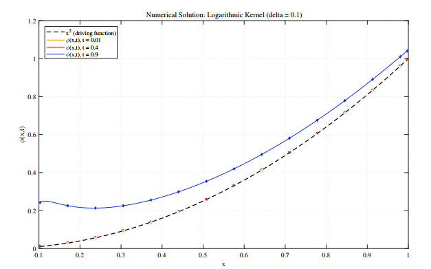
The numerical spatial solution $\phi(x, t)$ for the logarithmic kernel on $0.1\leq x\leq1$, using $n = 160$ positive-half cells, at $t = 0.01, 0.4, 0.9$. The dashed curve denotes $x^2$
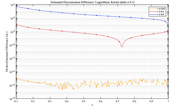
The estimated mesh-refinement difference $E_{160,320}(x_i, t) = |\phi_{160}(x_i, t)- \phi_{320}^{\mathrm{ext}}(x_i, t)|$ for the logarithmic kernel at $t = 0.01, 0.4, 0.9$. The refined solution is evaluated at coarse nodes; the vertical scale is logarithmic
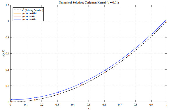
The spatial numerical solution $\phi(x, t)$ for the Carleman kernel with $p = 0.01$ and $n = 80$, at $t = 0.01, 0.4, 0.9$. The dashed curve denotes $x^2$
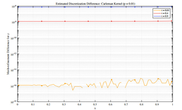
The estimated mesh-refinement difference $E_{80,160}(x_i, t) = |\phi_{80}(x_i, t)- \phi_{160}^{\mathrm{ext}}(x_i, t)|$ for the Carleman kernel with $p = 0.01$ at $t = 0.01, 0.4, 0.9$. The vertical scale is logarithmic
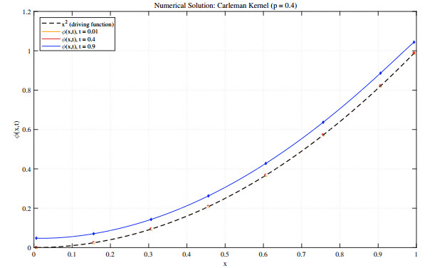
The numerical spatial solution $\phi(x, t)$ for the Carleman kernel with $p = 0.4$ and $n = 80$, at $t = 0.01, 0.4, 0.9$. The dashed curve denotes $x^2$
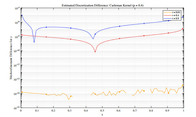
The estimated mesh-refinement difference $E_{80,160}(x_i, t) = |\phi_{80}(x_i, t)- \phi_{160}^{\mathrm{ext}}(x_i, t)|$ for the Carleman kernel with $p = 0.4$ at $t = 0.01, 0.4, 0.9$. The vertical scale is logarithmic
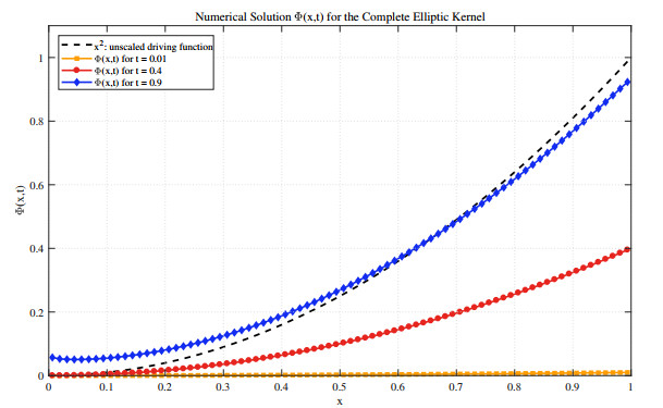
The numerical scaled solution $\Phi(x, t) = t\phi(x, t)$ for the complete elliptic kernel with $p = 1/2$, $q = 2$, $\mu = 1$, $n = 80$, at $t = 0.01, 0.4, 0.9$. The dashed curve represents the unscaled reference $x^2$, not the source $t x^2$
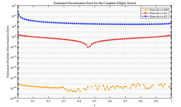
The estimated mesh-refinement difference $E_{80,160}(x_i, t) = |\Phi_{80}(x_i, t)- \Phi_{160}^{\mathrm{ext}}(x_i, t)|$ for the complete elliptic kernel with $p = 1/2$, $q = 2$, $\mu = 1$, at $t = 0.01, 0.4, 0.9$. The vertical scale is logarithmic; early-time differences are near floating-point roundoff
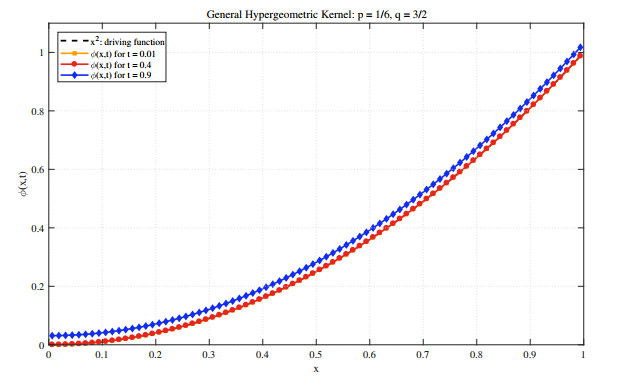
The numerical solution for the general hypergeometric kernel at different times for $(p, q) = \left(\frac{1}{6}, \frac{3}{2}\right)$. The curves represent $\phi(x, t)$ for $t = 0.01, 0.4, 0.9$, with $\mu = 1$ and $n = 80$
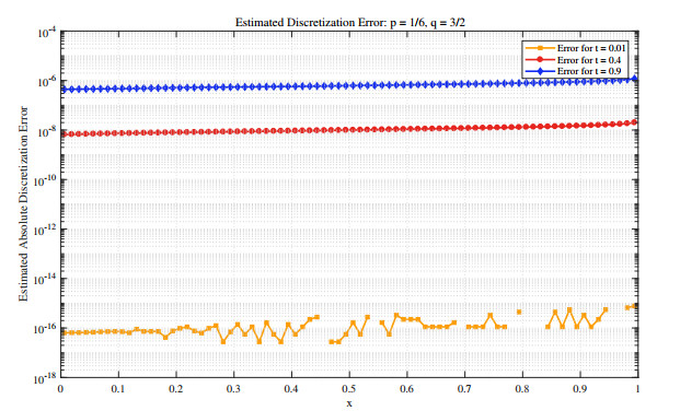
The estimated discretization error for the general hypergeometric kernel at different times for $(p, q) = \left(\frac{1}{6}, \frac{3}{2}\right)$. For $\mu = 1$ and $t = 0.01, 0.4, 0.9$, the plotted mesh-refinement difference is $E_{80,160}(x_i, t) = |\phi_{80}(x_i, t)-\phi_{160}^{\mathrm{ext}}(x_i, t)|$, where the refined solution is evaluated at the coarse-grid nodes. The vertical scale is logarithmic
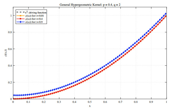
The numerical solution for the general hypergeometric kernel at different times for $(p, q) = (0.4, 2)$. The curves represent $\phi(x, t)$ for $t = 0.01, 0.4, 0.9$, with $\mu = 1$ and $n = 80$
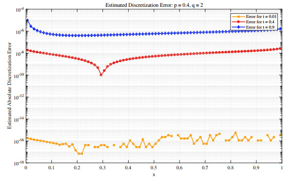
The estimated discretization error for the general hypergeometric kernel at different times for $(p, q) = (0.4, 2)$. For $\mu = 1$ and $t = 0.01, 0.4, 0.9$, the plotted mesh-refinement difference is $E_{80,160}(x_i, t) = |\phi_{80}(x_i, t)-\phi_{160}^{\mathrm{ext}}(x_i, t)|$, where the refined solution is evaluated at the coarse-grid nodes. The vertical scale is logarithmic




 DownLoad: