Using the spectral properties of orthogonal polynomials, we introduce an algebraic version of quantum field theory for elementary particles. The formulation enabled us to propose a model where closed-loop integrals in the Feynman diagrams for computing transition amplitudes are divergence-free. Consequently, the model is finite, and no renormalization scheme is required as in the conventional theory. It remains to be seen whether the finiteness property could be extended to other physically relevant models.
Citation: A. D. Alhaidari. Finite spectral quantum field theory[J]. AIMS Mathematics, 2026, 11(11): 37186-37219. doi: 10.3934/math.20261437
Using the spectral properties of orthogonal polynomials, we introduce an algebraic version of quantum field theory for elementary particles. The formulation enabled us to propose a model where closed-loop integrals in the Feynman diagrams for computing transition amplitudes are divergence-free. Consequently, the model is finite, and no renormalization scheme is required as in the conventional theory. It remains to be seen whether the finiteness property could be extended to other physically relevant models.

| [1] |
H. Epstein, V. Glaser, The role of locality in perturbation theory, Ann. Inst. Henri Poincaré, 19 (1973), 211–295. |
| [2] |
N. N. Bogoliubow, O. S. Parasiuk, Über die multiplikation der kausalfunktionen in der quantentheorie der Felder, Acta Math., 97 (1957), 227–266. https://doi.org/10.1007/BF02392399 doi: 10.1007/BF02392399
|
| [3] |
K. Hepp, Proof of the Bogoliubov-Parasiuk theorem on renormalization, Commun. Math. Phys., 2 (1966), 301–326. https://doi.org/10.1007/BF01773358 doi: 10.1007/BF01773358
|
| [4] |
W. Zimmermann, Convergence of Bogoliubov's method of renormalization in momentum space, Commun. Math. Phys., 15 (1969), 208–234. https://doi.org/10.1007/BF01645676 doi: 10.1007/BF01645676
|
| [5] |
Y. L. Wu, Quantum structure of field theory and Standard Model based on infinity-free loop regularization/renormalization, Int. J. Mod. Phys. A, 29 (2014), 1430007. https://doi.org/10.1142/S0217751X14300075 doi: 10.1142/S0217751X14300075
|
| [6] |
J. R. Klauder, Divergences in scalar quantum field theory: the cause and the cure, Mod. Phys. Lett. A, 27 (2012), 1250117. https://doi.org/10.1142/S0217732312501179 doi: 10.1142/S0217732312501179
|
| [7] |
P. Tillman, Ultraviolet-finite QFT on curved space-times, arXiv, 2010. https://doi.org/10.48550/arXiv.1009.1970 |
| [8] |
J. D. Bjorken, S. D. Drell, Relativistic quantum fields, McGraw-Hill College, 1965. |
| [9] |
C. Itzykson, J. B. Zuber, Quantum field theory, McGraw-Hill, 1980. |
| [10] |
N. N. Bogoliubov, D. V. Shirkov, Introduction to the theory of quantized fields, 3 Eds., John Wiley, 1980. |
| [11] |
G. Szegö, Orthogonal polynomials, American Mathematical Society, 1939. |
| [12] |
T. S. Chihara, An introduction to orthogonal polynomials, Gordon and Breach, 1978. |
| [13] |
M. E. H. Ismail, Classical and quantum orthogonal polynomials in one variable, Cambridge University Press, 2009. https://doi.org/10.1017/CBO9781107325982 |
| [14] |
A. D. Alhaidari, A. Laradji, A novel algebraic system in quantum field theory, Appl. Math., 3 (2023), 461–467. https://doi.org/10.3390/appliedmath3020024 doi: 10.3390/appliedmath3020024
|
| [15] |
A. D. Alhaidari, Structural algebraic quantum field theory: particles with structure, Phys. Part. Nuclei Lett., 20 (2023), 1293–1307. https://doi.org/10.1134/S154747712306002X doi: 10.1134/S154747712306002X
|
| [16] |
A. D. Alhaidari, Gauss quadrature for integrals and sums, Int. J. Pure Appl. Math. Res., 3 (2023), 1. https://doi.org/10.20944/preprints202302.0222.v1 doi: 10.20944/preprints202302.0222.v1
|
| [17] |
D. Damanik, A. Pushnitski, B. Simon, The analytic theory of matrix orthogonal polynomials, Surv. Approx. Theory, 4 (2008), 1. |
| [18] |
M. E. H. Ismail, E. Koelink, P. Román, Matrix valued Hermite polynomials, Burchnall formulas and non-abelian Toda lattice, Adv. Appl. Math., 110 (2019), 235–269. https://doi.org/10.1016/j.aam.2019.07.002 doi: 10.1016/j.aam.2019.07.002
|
| [19] |
E. Koelink, P. Román, W. Zudilin, An evolution of matrix-valued orthogonal polynomials, Pacific J. Math., 338 (2025), 325–348. https://doi.org/10.2140/pjm.2025.338.325 doi: 10.2140/pjm.2025.338.325
|
| [20] |
H. A. Yamani, Z. Mouayn, Properties of shape-invariant tridiagonal Hamiltonians, Theor. Math. Phys., 203 (2020), 761–779. https://doi.org/10.1134/S0040577920060057 doi: 10.1134/S0040577920060057
|
Figures(11) / Tables(1)

A. D. Alhaidari. Finite spectral quantum field theory[J]. AIMS Mathematics, 2026, 11(11): 37186-37219. doi: 10.3934/math.20261437

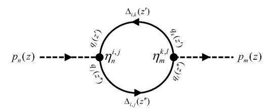
Feynman diagram for the first-order (single loop) correction to the scalar propagator (i.e., self-energy) in the model $ {L_I} = \eta \bullet \left[ {\Phi \, (\bar{ \mathcal{X}}\, \mathcal{X})} \right] $
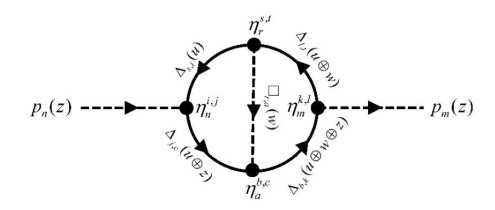
One of the Feynman diagrams contributing to the second-order (two-loop) correction to the scalar propagator (i.e., self-energy) in the model $ {L_I} = \eta \bullet \left[ {\Phi \, (\bar{ \mathcal{X}}\, \mathcal{X})} \right] $
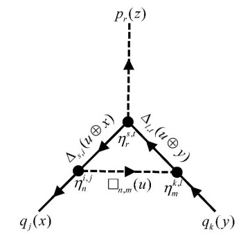
One of the Feynman diagrams contributing to the first-order (one-loop) correction to the interaction vertex $ \left\langle {{{p_r}(z)}} \mathrel{\left | {\vphantom {{{p_r}(z)} {{q_j}(x){q_k}(y)}}} \right. } {{{q_j}(x){q_k}(y)}} \right\rangle $ in the model $ {L_I} = \eta \bullet \left[ {\Phi \, (\bar{ \mathcal{X}}\, \mathcal{X})} \right] $
Gauss quadrature approximation of the integral (28) with a quadrature order $ \mathcal{M} = 100 $
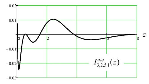
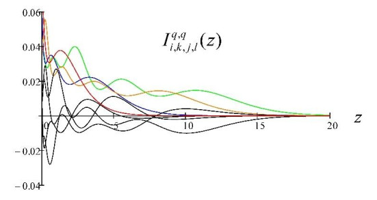
Plot of the integral (28) corresponding to monochrome propagation as $ \zeta _{2, 1}^{q, q}(z) $ in red, $ \zeta _{2, 5}^{q, q}(z) $ in green, $ \zeta _{3, 2}^{q, q}(z) $ in blue, and $ \zeta _{3, 4}^{q, q}(z) $ in brown. Plots in black correspond to polychrome propagation for $ I_{3, 2, 5, 4}^{q, q}(z) $, $ I_{2, 3, 4, 1}^{q, q}(z) $, $ I_{2, 4, 5, 3}^{q, q}(z) $, and $ I_{2, 1, 2, 5}^{q, q}(z) $
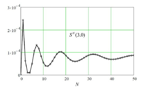
The partial sum $ {S^N}(z) $ defined by Eq (30) for $ \kappa = 1 $ and $ z = 3.0 $. The elements of the coupling tensor in this model are given by Eq (27)
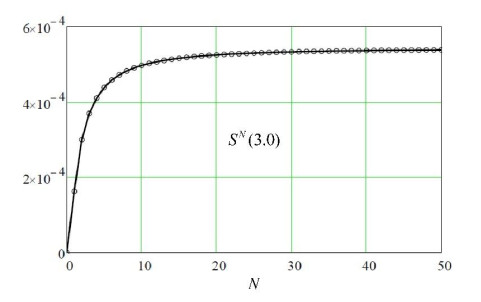
Reproduction of Figure 6 after imposing monochrome propagation
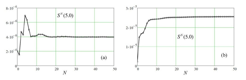
Reproduction of Figures 4 and 5 for the spinor particle but for $ z = 5.0 $: (a) polychrome propagation, (b) monochrome propagation
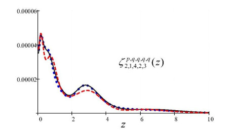
Plot of the integral (33) that demonstrates convergence by increasing the Gauss quadrature order from 15 (dashed red) to 20 (dotted blue) and to 30 (solid black)
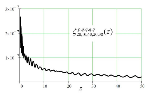
Reproduction of Figure 9 (with a Gauss quadrature order of 50) but for 10 times the values of the indices demonstrating diminishing values (of the order of 200 times less) where we used the asymptotic formula (34) for the spectral polynomials
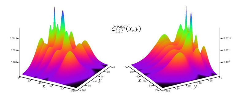
Two-dimensional plot of the integral (35) viewed from two different angles. The x-axis scale is 0.15, while the y-axis scale is 0.30




 DownLoad: