The number of fiber intersections $ Y $ inside a bounded counting region of a two-dimensional random fiber web is a lattice-valued statistic whose finite-sample distribution can be asymmetric in a way that the recently established Gaussian limit cannot represent. That, together with the overdispersion of $ Y $ above a geometry-dependent fiber-count threshold and the mismatch between a continuous law and a lattice, motivates the negative binomial law matched to the exact finite-sample mean and variance of $ Y $. We first showed that the conditional intersection probability depends on a partner fiber's seeding region only through its expected truncated length, so the moment formulas keep their form under type-specific seeding; this settles a question left open by Chun and Jhong (2026). We then provided the exact finite-sample threshold beyond which the moment-matched fit exists—weaker in our configuration than the leading-order condition by a factor of about $ 63 $—and settled which negative binomial parameter must diverge for asymptotic normality: Not $ r_n $, for which we give a counterexample, but $ r_n(1-\theta_n) $. A large-scale simulation then compared the two approximations on a common lattice, using closed-form truncated-length moments. Two corrections proved essential: The Kolmogorov–Smirnov statistic must be evaluated for a lattice reference law, and the normal law must carry a half-count continuity correction, which alone is worth some $ 60\% $ of the apparent gain. The negative binomial's remaining advantage is real but not uniform: A factor of two in Kolmogorov distance at $ 150 $ equal-length fibers, the same at $ 300 $ on weaker evidence, not resolved from $ 500 $ onward, and reversed in one mixture configuration. On the Kolmogorov distance restricted to the outer $ 10\% $ of the distribution, it was ahead in every configuration we ran, though not in every individual tail cell; at $ 150 $ fibers and three standard deviations, the corrected Gaussian understated the upper tail by a factor of $ 2.2 $ and the negative binomial by $ 15\% $.
Citation: Heuiju Chun, Jae-Hwan Jhong. A moment-matched negative binomial approximation for fiber intersection counts in two-dimensional random webs[J]. AIMS Mathematics, 2026, 11(11): 36134-36162. doi: 10.3934/math.20261400
The number of fiber intersections $ Y $ inside a bounded counting region of a two-dimensional random fiber web is a lattice-valued statistic whose finite-sample distribution can be asymmetric in a way that the recently established Gaussian limit cannot represent. That, together with the overdispersion of $ Y $ above a geometry-dependent fiber-count threshold and the mismatch between a continuous law and a lattice, motivates the negative binomial law matched to the exact finite-sample mean and variance of $ Y $. We first showed that the conditional intersection probability depends on a partner fiber's seeding region only through its expected truncated length, so the moment formulas keep their form under type-specific seeding; this settles a question left open by Chun and Jhong (2026). We then provided the exact finite-sample threshold beyond which the moment-matched fit exists—weaker in our configuration than the leading-order condition by a factor of about $ 63 $—and settled which negative binomial parameter must diverge for asymptotic normality: Not $ r_n $, for which we give a counterexample, but $ r_n(1-\theta_n) $. A large-scale simulation then compared the two approximations on a common lattice, using closed-form truncated-length moments. Two corrections proved essential: The Kolmogorov–Smirnov statistic must be evaluated for a lattice reference law, and the normal law must carry a half-count continuity correction, which alone is worth some $ 60\% $ of the apparent gain. The negative binomial's remaining advantage is real but not uniform: A factor of two in Kolmogorov distance at $ 150 $ equal-length fibers, the same at $ 300 $ on weaker evidence, not resolved from $ 500 $ onward, and reversed in one mixture configuration. On the Kolmogorov distance restricted to the outer $ 10\% $ of the distribution, it was ahead in every configuration we ran, though not in every individual tail cell; at $ 150 $ fibers and three standard deviations, the corrected Gaussian understated the upper tail by a factor of $ 2.2 $ and the negative binomial by $ 15\% $.

| [1] |
O. Kallmes, H. Corte, The structure of paper. Ⅰ. The statistical geometry of an ideal two dimensional fiber network, Tappi J., 43 (1960), 737–752. |
| [2] |
T. Komori, Y. Ujihara, Y. Matsunaga, K. Makishima, Crossings of curled fibers in two-dimensional assemblies, Tappi, 62 (1979), 93–95. |
| [3] |
Y. B. Yi, L. Berhan, A. M. Sastry, Statistical geometry of random fibrous networks, revisited: Waviness, dimensionality, and percolation, J. Appl. Phys., 96 (2004), 1318–1327. https://doi.org/10.1063/1.1763240 doi: 10.1063/1.1763240
|
| [4] |
M. W. Suh, H. Chun, R. L. Berger, P. Bloomfield, Distribution of fiber intersections in two-dimensional random fiber webs–A basic geometrical probability model, Text. Res. J., 80 (2010), 301–311. https://doi.org/10.1177/0040517509105071 doi: 10.1177/0040517509105071
|
| [5] |
H. Chun, Probabilistic modeling of fiber length segments within a bounded area of two-dimensional fiber webs, Commun. Stat. Appl. Met., 18 (2011), 301–317. https://doi.org/10.5351/CKSS.2011.18.3.301 doi: 10.5351/CKSS.2011.18.3.301
|
| [6] |
H. Chun, M. W. Suh, Distribution of fiber intersections in two-dimensional random fiber web cases with a mixture of two fiber lengths, Text. Res. J., 90 (2020), 1851–1859. https://doi.org/10.1177/0040517519898158 doi: 10.1177/0040517519898158
|
| [7] |
H. Chun, J. H. Jhong, Asymptotic distribution of fiber intersection counts in two-dimensional random fiber webs, AIMS Math., 11 (2026), 15008–15027. https://doi.org/10.3934/math.2026617 doi: 10.3934/math.2026617
|
| [8] |
Y. Wang, B. Zhou, C. Fu, X. Xu, Modeling cure fractions in interval-censored competing risks data: An AFT mixture approach, Electron. Res. Arch., 34 (2026), 6573–6613. https://doi.org/10.3934/era.2026288 doi: 10.3934/era.2026288
|
| [9] |
P. C. Consul, G. C. Jain, A generalization of the Poisson distribution, Technometrics, 15 (1973), 791–799. https://doi.org/10.1080/00401706.1973.10489112 doi: 10.1080/00401706.1973.10489112
|
| [10] |
R. W. Conway, W. L. Maxwell, A queuing model with state dependent service rates, J. Ind. Eng., 12 (1962), 132–136. |
| [11] |
G. Shmueli, T. P. Minka, J. B. Kadane, S. Borle, P. Boatwright, A useful distribution for fitting discrete data: Revival of the Conway–Maxwell–Poisson distribution, J. R. Stat. Soc. C-Appl., 54 (2005), 127–142. https://doi.org/10.1111/j.1467-9876.2005.00474.x doi: 10.1111/j.1467-9876.2005.00474.x
|
| [12] |
A. D. Barbour, L. Holst, S. Janson, Poisson approximation, Oxford: Oxford University Press, 1992. https://doi.org/10.1093/oso/9780198522355.001.0001 |
| [13] |
M. H. Quenouille, A relation between the logarithmic, Poisson, and negative binomial series, Biometrics, 5 (1949), 162–164. https://doi.org/10.2307/3001917 doi: 10.2307/3001917
|
| [14] |
N. L. Johnson, A. W. Kemp, S. Kotz, Univariate discrete distributions, 3 Eds., Hoboken: Wiley, 2005. https://doi.org/10.1002/0471715816 |
| [15] |
F. Ouimet, A refined continuity correction for the negative binomial distribution and asymptotics of the median, Metrika, 86 (2023), 827–849. https://doi.org/10.1007/s00184-023-00897-2 doi: 10.1007/s00184-023-00897-2
|
| [16] |
T. C. Brown, M. J. Phillips, Negative binomial approximation with Stein's method, Methodol. Comput. Appl., 1 (1999), 407–421. https://doi.org/10.1023/A:1010094221471 doi: 10.1023/A:1010094221471
|
| [17] |
A. D. Barbour, H. L. Gan, A. Xia, Stein factors for negative binomial approximation in Wasserstein distance, Bernoulli, 21 (2015), 1002–1013. https://doi.org/10.3150/14-BEJ595 doi: 10.3150/14-BEJ595
|
| [18] |
Y. D. Liang, B. A. Barsky, A new concept and method for line clipping, ACM T. Graphic., 3 (1984), 1–22. https://doi.org/10.1145/357332.357333 doi: 10.1145/357332.357333
|
| [19] |
D. S. Dimitrova, V. K. Kaishev, S. Tan, Computing the Kolmogorov–Smirnov distribution when the underlying cdf is purely discrete, mixed, or continuous, J. Stat. Softw., 95 (2020), 1–42. https://doi.org/10.18637/jss.v095.i10 doi: 10.18637/jss.v095.i10
|
| [20] |
H. Callaert, P. Janssen, The Berry–Esseen theorem for $U$-statistics, Ann. Stat., 6 (1978), 417–421. https://doi.org/10.1214/aos/1176344132 doi: 10.1214/aos/1176344132
|
| [21] |
V. S. Korolyuk, Y. V. Borovskich, Theory of $U$-statistics, In: Mathematics and Its Applications, Dordrecht: Springer, 1994. https://doi.org/10.1007/978-94-017-3515-5 |
| [22] |
P. J. Bickel, F. Götze, W. R. V. Zwet, The Edgeworth expansion for $U$-statistics of degree two, Ann. Stat., 14 (1986), 1463–1484. https://doi.org/10.1214/aos/1176350170 doi: 10.1214/aos/1176350170
|
| [23] |
V. Bentkus, F. Götze, W. R. V. Zwet, An Edgeworth expansion for symmetric statistics, Ann. Stat., 25 (1997), 851–896. https://doi.org/10.1214/aos/1031833676 doi: 10.1214/aos/1031833676
|
| [24] |
W. Wang, H. Wu, Z. Dai, W. Liu, Distributed optimal subsampling inference for the additive hazards model with massive survival data, BMC Med. Res. Methodol., 2026. https://doi.org/10.1186/s12874-026-02985-z doi: 10.1186/s12874-026-02985-z
|
Figures(3) / Tables(6)

Heuiju Chun, Jae-Hwan Jhong. A moment-matched negative binomial approximation for fiber intersection counts in two-dimensional random webs[J]. AIMS Mathematics, 2026, 11(11): 36134-36162. doi: 10.3934/math.20261400

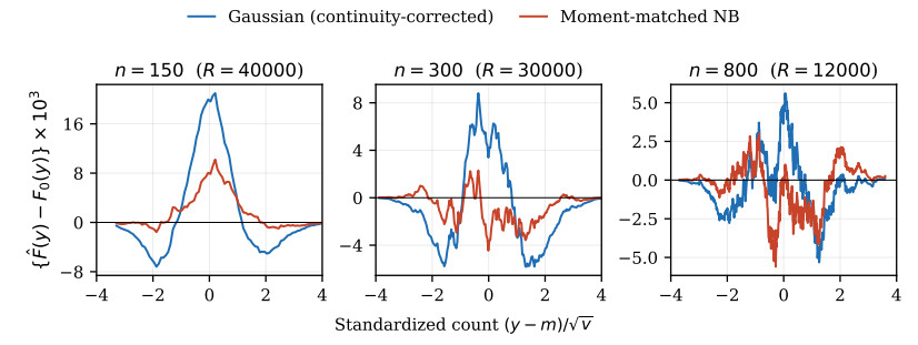
Difference between the simulated distribution function of $ Y $ and each approximation, against the standardized count. Both approximations are built from the same finite-$ n $ moments $ (m, v) $ and so differ only in shape
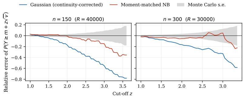
Relative error of the approximate upper-tail probability $ \mathbb{P}(Y\ge m+z\sqrt v) $ as a function of the cut-off $ z $, for two fiber counts, shown only as far out as the simulation resolves (at least $ 25 $ observed exceedances in the simulation). The shaded band is one estimated relative Monte Carlo standard error of the simulated tail probability, on either side of zero; it is not a confidence band for either approximation curve. The symmetric Gaussian approximation understates the upper tail increasingly severely as $ z $ grows. The negative binomial reduces that underestimation over the whole of the displayed range, by a factor of roughly two at the largest cut-offs, but does not remove it: Its own relative error is negative and growing at the edge of resolution
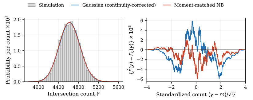
Two-length mixture model under type-specific seeding. Left: The simulated distribution of $ Y $ with the two lattice approximations overlaid. Right: The difference between the simulated distribution function and each approximation, as in Figure 1




 DownLoad: