Deep learning approaches for $ \beta- $conformable fractional differential equations: A PINN, NRPINN-s, and NRPINN-un based solutions

Sadullah Bulut; Muhammed Yiğider; Sadullah Bulut; Muhammed Yiğider

doi:10.3934/math.2025618

AIMS Mathematics

2025, Volume 10, Issue 6: 13721-13740. doi: 10.3934/math.2025618

Previous Article Next Article

Research article

Deep learning approaches for $ \beta- $conformable fractional differential equations: A PINN, NRPINN-s, and NRPINN-un based solutions

Sadullah Bulut ,
Muhammed Yiğider ^,

Department of Mathematics, Erzurum Technical University, Yakutiye, Erzurum 25050, Turkey

Received: 18 February 2025 Revised: 30 May 2025 Accepted: 04 June 2025 Published: 13 June 2025
MSC : 65M50, 35R11, 68T07

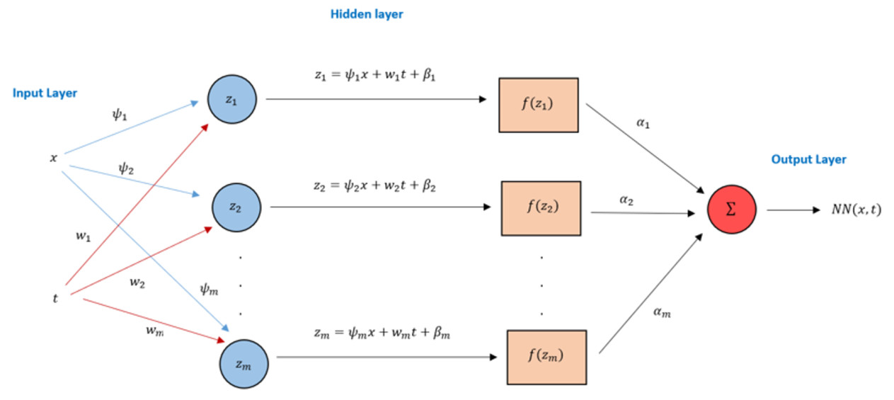
In this paper, we present a numerical approach for solving $ \beta- $conformable fractional differential equations (FDEs) using physics-informed neural networks (PINNs) and their enhanced versions, NRPINN-s and NRPINN-un. The proposed method combines the flexibility of artificial neural networks with the inherent structure of fractional calculus, allowing the solution of complex initial and boundary value problems without domain discretization. The loss function in the model includes initial and boundary conditions and is constructed using modifiable parameters (weights and biases). The efficiency of the proposed methods is demonstrated by numerical experiments on heat and wave equations. The obtained results show that NR-PINNs are superior to classical PINNs in improving convergence, reducing local errors and showing good performance. Visual and tabular comparisons of the solutions obtained from the method with analytical solutions confirm the effectiveness of the approach.
- Physics-Informed Neural Networks (PINNs),
- $ \beta- $conformable fractional differential equations,
- NR-PINN,
- deep learning
Citation: Sadullah Bulut, Muhammed Yiğider. Deep learning approaches for $ \beta- $conformable fractional differential equations: A PINN, NRPINN-s, and NRPINN-un based solutions[J]. AIMS Mathematics, 2025, 10(6): 13721-13740. doi: 10.3934/math.2025618

Related Papers:

Abstract

In this paper, we present a numerical approach for solving $ \beta- $conformable fractional differential equations (FDEs) using physics-informed neural networks (PINNs) and their enhanced versions, NRPINN-s and NRPINN-un. The proposed method combines the flexibility of artificial neural networks with the inherent structure of fractional calculus, allowing the solution of complex initial and boundary value problems without domain discretization. The loss function in the model includes initial and boundary conditions and is constructed using modifiable parameters (weights and biases). The efficiency of the proposed methods is demonstrated by numerical experiments on heat and wave equations. The obtained results show that NR-PINNs are superior to classical PINNs in improving convergence, reducing local errors and showing good performance. Visual and tabular comparisons of the solutions obtained from the method with analytical solutions confirm the effectiveness of the approach.

References

[1]	Y. Zhao, J. Xia, X. Lü, The variable separation solution, fractal and chaos in an extended coupled (2+ 1)-dimensional Burgers system, Nonlinear Dynam., 108 (2022), 4195–4205. https://doi.org/10.1007/s11071-021-07100-z doi: 10.1007/s11071-021-07100-z
[2]	A. Akbulut, S. Islam, Study on the Biswas–Arshed equation with the beta time derivative, Int. J. Appl. Computat. Math., 8 (2022), article number 167. https://doi.org/10.1007/s40819-022-01350-0 doi: 10.1007/s40819-022-01350-0
[3]	M. Cinar, A. Secer, M. Ozisik, M. Bayram, Derivation of optical solitons of dimensionless Fokas-Lenells equation with perturbation term using Sardar sub-equation method, Opt. Quant. Electron., 54 (2022), article number 402. https://doi.org/10.1007/s11082-022-03819-0 doi: 10.1007/s11082-022-03819-0
[4]	S. Kumar, M. Niwas, New optical soliton solutions of Biswas–Arshed equation using the generalised exponential rational function approach and Kudryashov's simplest equation approach, Pramana, 96 (2022), 204. https://doi.org/10.1007/s12043-022-02450-8 doi: 10.1007/s12043-022-02450-8
[5]	K. Wang, Bäcklund transformation and diverse exact explicit solutions of the fractal combined Kdv–mkdv equation, Fractals, 30 (2022), 2250189. https://doi.org/10.1142/S0218348X22501894 doi: 10.1142/S0218348X22501894
[6]	M. Ghayad, N. Badra, H. Ahmed, W. Rabie, Derivation of optical solitons and other solutions for nonlinear Schrödinger equation using modified extended direct algebraic method, Alex. Eng. J., 64 (2023), 801–811. https://doi.org/10.1016/j.aej.2022.10.054 doi: 10.1016/j.aej.2022.10.054
[7]	M. Hashemi, M. Mirzazadeh, Optical solitons of the perturbed nonlinear Schrödinger equation using Lie symmetry method, Optik, 281 (2023), 170816. https://doi.org/10.1016/j.ijleo.2023.170816 doi: 10.1016/j.ijleo.2023.170816
[8]	J. Martin, S. Duncan, A Galerkin approach for modelling the pantograph-catenary interaction, Advances In Dynamics Of Vehicles On Roads And Tracks: Proceedings Of The 26th Symposium Of The International Association Of Vehicle System Dynamics, IAVSD 2019, August 12–16, 2019, Gothenburg, Sweden, 230–241, (2020). https://doi.org/10.1007/978-3-030-38077-9
[9]	F. Mariano, L. Moreira, A. Nascimento, A. Silveira-Neto, An improved immersed boundary method by coupling of the multi-direct forcing and Fourier pseudo-spectral methods, J. Braz. Soc. Mech. Sci., 44 (2022), 388. https://doi.org/10.1007/s40430-022-03679-5 doi: 10.1007/s40430-022-03679-5
[10]	A. Hussain, M. Junaid-U-Rehman, F. Jabeen, I. Khan, Optical solitons of NLS-type differential equations by extended direct algebraic method. Int. J. Geom. Methods M., 19 (2022), 2250075. https://doi.org/https://doi.org/10.1142/S021988782250075X
[11]	M. Ali, H. El-Owaidy, H. Ahmed, A. El-Deeb, I. Samir, Optical solitons and complexitons for generalized Schrödinger–Hirota model by the modified extended direct algebraic method, Opt. Quant. Electron., 55 (2023), 675. https://doi.org/10.1007/s11082-023-04962-y doi: 10.1007/s11082-023-04962-y
[12]	W. Ma, Y. Zhang, Y. Tang, Symbolic computation of lump solutions to a combined equation involving three types of nonlinear terms, East Asian J. Appl. Math., 10 (2020), 732–745. https://doi.org/10.4208/eajam.151019.110420 doi: 10.4208/eajam.151019.110420
[13]	Y. Gu, S. Zia, M. Isam, J. Manafian, A. Hajar, M. Abotaleb, Bilinear method and semi-inverse variational principle approach to the generalized (2+ 1)-dimensional shallow water wave equation, Results Phys., 45 (2023), 106213. https://doi.org/10.1016/j.rinp.2023.106213 doi: 10.1016/j.rinp.2023.106213
[14]	A. Yokus, M. Isah, Dynamical behaviors of different wave structures to the Korteweg–de Vries equation with the Hirota bilinear technique, Physica A, 622 (2023), 128819. https://doi.org/10.1016/j.physa.2023.128819 doi: 10.1016/j.physa.2023.128819
[15]	Y. Shen, B. Tian, T. Zhou, X. Gao, N-fold Darboux transformation and solitonic interactions for the Kraenkel–Manna–Merle system in a saturated ferromagnetic material, Nonlinear Dynam., 111 (2023), 2641–2649. https://doi.org/10.1007/s11071-022-07959-6 doi: 10.1007/s11071-022-07959-6
[16]	T. Yin, Z. Xing, J. Pang, Modified Hirota bilinear method to (3+ 1)-D variable coefficients generalized shallow water wave equation, Nonlinear Dynam., 111 (2023), 9741–9752. https://doi.org/10.1007/s11071-023-08356-3 doi: 10.1007/s11071-023-08356-3
[17]	A. Hussain, Y. Chahlaoui, F. Zaman, T. Parveen, A. Hassan, The Jacobi elliptic function method and its application for the stochastic NNV system, Alex. Eng. J., 81 (2023), 347–359. https://doi.org/10.1016/j.aej.2023.09.017 doi: 10.1016/j.aej.2023.09.017
[18]	P. Das, S. Mirhosseini-Alizamini, D. Gholami, H. Rezazadeh, A comparative study between obtained solutions of the coupled Fokas–Lenells equations by Sine-Gordon expansion method and rapidly convergent approximation method, Optik, 283 (2023), 170888. https://doi.org/10.1016/j.ijleo.2023.170888 doi: 10.1016/j.ijleo.2023.170888
[19]	E. Fan, H. A. Zhang, Note on the homogeneous balance method, Phys. Lett. A, 246 (1998), 403–406. https://doi.org/https://doi.org/10.1016/S0375-9601(98)00547-7 doi: 10.1016/S0375-9601(98)00547-7
[20]	A. Yokus, M. Isah, Stability analysis and solutions of (2+ 1)-Kadomtsev–Petviashvili equation by homoclinic technique based on Hirota bilinear form, Nonlinear Dynam., 109 (2022), 3029–3040. https://doi.org/10.1007/s11071-022-07568-3 doi: 10.1007/s11071-022-07568-3
[21]	K. Fatema, M. Islam, M. Akhter, M. Akbar, M. Inc, Transcendental surface wave to the symmetric regularized long-wave equation, Phys. Lett. A, 439 (2022), 128123. https://doi.org/https://doi.org/10.1016/j.physleta.2022.128123 doi: 10.1016/j.physleta.2022.128123
[22]	M. Kaplan, A. Bekir, A. Akbulut, E. Aksoy, The modified simple equation method for nonlinear fractional differential equations, Rom. J. Phys., 60 (2015), 1374–1383.
[23]	G. Gie, C. Jung, H. Lee, Semi-analytic shooting methods for Burgers' equation, J. Comput. Appl. Math., 418 (2023), 114694. https://doi.org/https://doi.org/10.1016/j.cam.2022.114694 doi: 10.1016/j.cam.2022.114694
[24]	S. Kiliç, E. Çelik, Complex solutions to the higher-order nonlinear boussinesq type wave equation transform, Ric. Mat., (2022), 1–8. https://doi.org/10.1007/s11587-022-00698-1
[25]	S. Kılıç, E. Çelik, H. Bulut, Solitary wave solutions to some nonlinear conformable partial differential equations, Opt. Quant. Electron., 55 (2023), 693. https://doi.org/10.1007/s11082-023-04983-7 doi: 10.1007/s11082-023-04983-7
[26]	T. Yazgan, E. Ilhan, E. Çelik, H. Bulut, On the new hyperbolic wave solutions to Wu-Zhang system models, Opt. Quant. Electron., 54 (2022), 298. https://doi.org/10.21203/rs.3.rs-1184408/v1 doi: 10.21203/rs.3.rs-1184408/v1
[27]	H. Lee, I. Kang, Neural algorithm for solving differential equations, J. Comput. Phys., 91 (1990), 110–131. https://doi.org/https://doi.org/10.1016/0021-9991(90)90007-N doi: 10.1016/0021-9991(90)90007-N
[28]	R. Gladstone, M. Nabian, N. Sukumar, A. Srivastava, H. Meidani, FO-PINN: A First-Order formulation for Physics-Informed Neural Networks, Eng. Anal. Bound. Elem., 174 (2025), 106161. https://doi.org/10.1016/j.enganabound.2025.106161 doi: 10.1016/j.enganabound.2025.106161
[29]	M. Vellappandi, S. Lee, Physics-informed Neural Fractional Differential Equations, Appl. Math. Model., (2025), 116127. https://doi.org/10.1016/j.apm.2025.116127
[30]	M. Zhong, S. Gong, S. Tian, Z. Yan, Data-driven rogue waves and parameters discovery in nearly integrable PT-symmetric Gross–Pitaevskii equations via PINNs deep learning, Physica D, 439 (2022), 133430. https://doi.org/10.1016/j.physd.2022.133430 doi: 10.1016/j.physd.2022.133430
[31]	K. Eshkofti, S. Hosseini, A new modified deep learning technique based on physics-informed neural networks (PINNs) for the shock-induced coupled thermoelasticity analysis in a porous material, J. Therm. Stresses, 47 (2024), 798–825. https://doi.org/10.1080/01495739.2024.2321205 doi: 10.1080/01495739.2024.2321205
[32]	M. Raissi, P. Perdikaris, G. Karniadakis, Physics-informed neural networks: A deep learning framework for solving forward and inverse problems involving nonlinear partial differential equations, J. Comput. Phys., 378 (2019), 686–707. https://doi.org/10.1016/j.jcp.2018.10.045 doi: 10.1016/j.jcp.2018.10.045
[33]	Z. Zhou, Z. Yan, Deep learning neural networks for the third-order nonlinear Schrödinger equation: bright solitons, breathers, and rogue waves, Commun. Theor. Phys., 73 (2021), 105006. https://doi.org/10.48550/arXiv.2104.14809 doi: 10.48550/arXiv.2104.14809
[34]	J. Song, Z. Yan, Deep learning soliton dynamics and complex potentials recognition for 1D and 2D PT-symmetric saturable nonlinear Schrödinger equations, Physica D, 448 (2023), 133729. https://doi.org/10.1016/j.physd.2023.133729 doi: 10.1016/j.physd.2023.133729
[35]	B. Zimmering, C. Coelho, O. Niggemann, Optimising neural fractional differential equations for performance and efficiency, Proc. Mach. Learn. Res., 255 (2024), 23.
[36]	G. Pang, M. D'Elia, M. Parks, G. Karniadakis, nPINNs: Nonlocal physics-informed neural networks for a parametrized nonlocal universal Laplacian operator, Algorithms and applications, J. Comput. Phys., 422 (2020), 109760. https://doi.org/10.1016/j.jcp.2020.109760 doi: 10.1016/j.jcp.2020.109760
[37]	M. D'Elia, M. Parks, G. Pang, G. Karniadakis, Nonlocal Physics-Informed Neural Networks: A unified theoretical and computational framework for nonlocal models, (Sandia National Lab.(SNL-NM), Albuquerque, NM (United States), 2020). https://doi.org/10.48550/arXiv.2004.04276
[38]	L. Lu, X. Meng, S. Cai, Z. Mao, S. Goswami, Z. Zhang, et al., Comprehensive and fair comparison of two neural operators (with practical extensions) based on fair data, Comput. Meth. Appl. Mech. Eng., 393 (2022), 114778. https://doi.org/10.1016/j.cma.2022.114778 doi: 10.1016/j.cma.2022.114778
[39]	A. Atangana, Derivative with a new parameter: Theory, methods and applications, (Academic Press, 2015).
[40]	R. Khalil, M. Al Horani, A. Yousef, M. Sababheh, A new definition of fractional derivative, J. Comput. Appl. Math. 264 (2014), 65–70. https://doi.org/10.1016/j.cam.2014.01.002 doi: 10.1016/j.cam.2014.01.002

Reader Comments

Your name:*

Email:*
© 2025 the Author(s), licensee AIMS Press. This is an open access article distributed under the terms of the Creative Commons Attribution License (http://creativecommons.org/licenses/by/4.0)