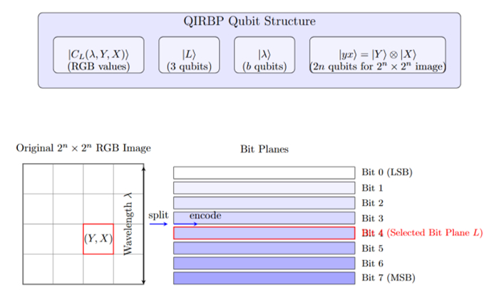
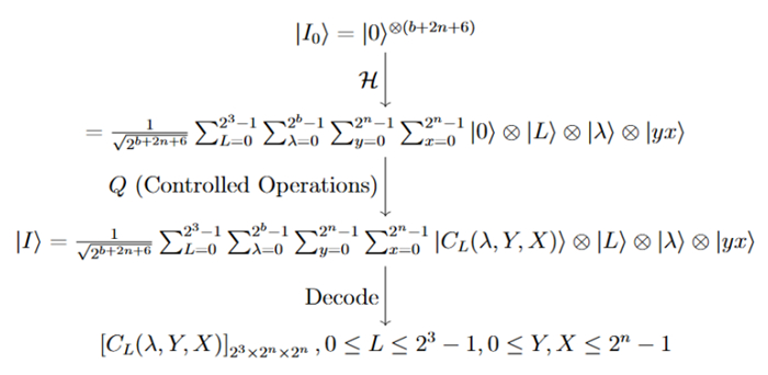
Quantum image processing (QIP) has become one of the most significant fields in quantum computing (QC); it merges quantum mechanics with image processing to improve classical image-processing speed, which involves various operations to advance quantum image representation (QIR). Accordingly, we introduce two new QIRs: The first is based on the wavelength and bit plane, called the quantum image representation bit plane (QIRBP), and the second is based on the wavelength and adjacency pixels, which is called the quantum image representation wavelength correlation (QIRWC). The QIRBP model uses $ b+2n+6 $ quantum bit (qubits) to store a digital color image of size $ {2}^{n}\times {2}^{n} $. In contrast, the QIRWC needs $ 2b+4n+8 $ qubits to store a digital color image of size $ {2}^{n}\times {2}^{n} $ and to entangle the wavelength between two neighboring pixels. While the QIRWC approach is more complex, it is also more efficient on the basis of the transformation data. The complexity arises from the level of information being transmitted. In this work, two new representation methods (QIRBP and QIRWC) are proposed to overcome existing QIR weaknesses by enhancing storage efficiency, enabling compact high-resolution representation, improving data transformation through wavelength correlation and pixel adjacency, reducing noise, achieving greater versatility, and advancing scalable QIR. To prove the efficiency of the proposed methods, they were analyzed and compared with other efficient quantum image representations, outlining their similar and different aspects.
Citation: Nawres A. Alwan, Suzan J. Obaiys, Nadia M. G. Al-Saidi, Nurul Fazmidar Binti Mohd Noor, Yeliz Karaca. A multi-channel quantum image representation model with qubit sequences for quantum-inspired image and image retrieval[J]. AIMS Mathematics, 2025, 10(5): 10994-11035. doi: 10.3934/math.2025499
Quantum image processing (QIP) has become one of the most significant fields in quantum computing (QC); it merges quantum mechanics with image processing to improve classical image-processing speed, which involves various operations to advance quantum image representation (QIR). Accordingly, we introduce two new QIRs: The first is based on the wavelength and bit plane, called the quantum image representation bit plane (QIRBP), and the second is based on the wavelength and adjacency pixels, which is called the quantum image representation wavelength correlation (QIRWC). The QIRBP model uses $ b+2n+6 $ quantum bit (qubits) to store a digital color image of size $ {2}^{n}\times {2}^{n} $. In contrast, the QIRWC needs $ 2b+4n+8 $ qubits to store a digital color image of size $ {2}^{n}\times {2}^{n} $ and to entangle the wavelength between two neighboring pixels. While the QIRWC approach is more complex, it is also more efficient on the basis of the transformation data. The complexity arises from the level of information being transmitted. In this work, two new representation methods (QIRBP and QIRWC) are proposed to overcome existing QIR weaknesses by enhancing storage efficiency, enabling compact high-resolution representation, improving data transformation through wavelength correlation and pixel adjacency, reducing noise, achieving greater versatility, and advancing scalable QIR. To prove the efficiency of the proposed methods, they were analyzed and compared with other efficient quantum image representations, outlining their similar and different aspects.

| [1] | R. P. Feynman, Simulating physics with computers, Feynman and computation, CRC Press, 2018,133–153. https://doi.org/10.1007/BF02650179 |
| [2] | P. W. Shor, Algorithms for quantum computation: Discrete logarithms and factoring, In: Proceedings 35th annual symposium on foundations of computer science, IEEE, 1994,124–134. https://doi.org/10.1109/SFCS.1994.365700 |
| [3] | L. K. Grover, A fast quantum mechanical algorithm for database search, In: Proceedings of the twenty-eighth annual ACM symposium on Theory of computing, 1996,212–219. https://doi.org/10.1145/237814.237866 |
| [4] | M. A. Nielsen, I. Chuang, Quantum computation and quantum information, American Association of Physics Teachers, Cambridge University Press, 2002. https://doi.org/10.1017/CBO9780511976667 |
| [5] |
J. He, H. Zhu, X. Zhou, Quantum image encryption algorithm via optimized quantum circuit and parity bit-planepermutation, J. Inf. Secur. Appl., 81 (2024), 103698. https://doi.org/10.1016/j.jisa.2024.103698 doi: 10.1016/j.jisa.2024.103698

|
| [6] |
J. Balewski, M. G. Amankwah, R. V. Beeumen, E. W. Bethel, T. Perciano, D. Camps, Quantum-parallel vectorized data encodings and computations on trapped-ion and transmon QPUs, Sci. Rep., 14 (2024), 3435. https://doi.org/10.1038/s41598-024-53720-x doi: 10.1038/s41598-024-53720-x
|
| [7] |
I. Attri, L. K. Awasthi, T. P. Sharma, EQID: Entangled quantum image descriptor an approach for early plant disease detection, Crop Prot., 188 (2025), 107005. https://doi.org/10.1016/j.cropro.2024.107005 doi: 10.1016/j.cropro.2024.107005
|
| [8] | H. Kumar, T. Ali, C. J. Holder, A. S. McGough, D. Bhowmik, Remote sensing classification using quantum image processing, Artificial Intelligence and Image and Signal Processing for Remote Sensing XXX, SPIE, 2024,157–169. https://doi.org/10.1117/12.3034036 |
| [9] |
S. Das, J. Zhang, S. Martina, D. Suter, F. Caruso, Quantum pattern recognition on real quantum processing units, Quant. Mach. Intell., 5 (2023), 16. https://doi.org/10.1007/s42484-022-00093-x doi: 10.1007/s42484-022-00093-x
|
| [10] | M. Marghany, Synthetic aperture radar image processing algorithms for nonlinear oceanic turbulence and front modeling, Elsevier, 2024. https://doi.org/10.1016/C2022-0-01174-0 |
| [11] |
P. Q. Le, F. Dong, K. Hirota, A flexible representation of quantum images for polynomial preparation, image compression, and processing operations, Quantum Inf. Process., 10 (2011), 63–84. https://doi.org/10.1007/s11128-010-0177-y doi: 10.1007/s11128-010-0177-y
|
| [12] |
J. Mu, X. Li, X. Zhang, P. Wang, Quantum implementation of the classical guided image filtering algorithm, Sci. Rep., 15 (2025), 493. https://doi.org/10.1038/s41598-024-84211-8 doi: 10.1038/s41598-024-84211-8
|
| [13] | M. R. Chowdhury, M. M. Islam, T. A. Sadi, M. H. H. Miraz, M. Mahdy, Edge detection quantumized: A novel quantum algorithm for image processing, arXiv Preprint, 2024. https://doi.org/10.48550/arXiv.2404.06889 |
| [14] |
T. Li, P. Zhao, Y. Zhou, Y. Zhang, Quantum image processing algorithm using line detection mask based on NEQR, Entropy, 25 (2023), 738. https://doi.org/10.3390/e25050738 doi: 10.3390/e25050738
|
| [15] | R. C. Gonzalez, R. E. Woods, S. L. Eddins, Digital image processing, publishing house of electronics industry, Beijing, China, 2002,262. |
| [16] | X. Fu, M. Ding, Y. Sun, S. Chen, A new quantum edge detection algorithm for medical images, MIPPR 2009: Medical imaging, parallel processing of images, and optimization techniques, SPIE, 2009,547–553. https://doi.org/10.1117/12.832499 |
| [17] |
H. S. Li, P. Fan, H. Y. Xia, H. Peng, S. Song, Quantum implementation circuits of quantum signal representation and type conversion, IEEE T. Circuits-I, 66 (2018), 341–354. http://doi.org/10.1109/TCSI.2018.2853655 doi: 10.1109/TCSI.2018.2853655
|
| [18] |
P. Benioff, The computer as a physical system: A microscopic quantum mechanical Hamiltonian model of computers as represented by Turing machines, J. Stat. Phys., 22 (1980), 563–591. https://doi.org/10.1007/BF01011339 doi: 10.1007/BF01011339
|
| [19] |
H. S. Li, S. Song, P. Fan, H. Peng, H. Y. Xia, Y. Liang, Quantum vision representations and multi-dimensional quantum transforms, Inform. Sciences, 502 (2019), 42–58. https://doi.org/10.1016/j.ins.2019.06.037 doi: 10.1016/j.ins.2019.06.037
|
| [20] | M. Nielsen, I. Chuang, Quantum computation and quantum information, Cambridge University Press, 2000. https://doi.org/10.1017/CBO9780511976667 |
| [21] |
S. E. V. Andraca, S. Bose, Storing, processing, and retrieving an image using quantum mechanics, Quantum Inf. Comput., 2003,137–147. https://doi.org/10.1117/12.485960 doi: 10.1117/12.485960
|
| [22] | J. I. Latorre, Image compression and entanglement, arXiv Preprint, 2005. https://doi.org/10.48550/arXiv.quant-ph/0510031 |
| [23] |
S. E. V. Andraca, J. Ball, Processing images in entangled quantum systems, Quantum Inf. Process., 9 (2010), 1–11. https://doi.org/10.1007/s11128-009-0123-z doi: 10.1007/s11128-009-0123-z
|
| [24] |
Y. Zhang, K. Lu, Y. Gao, M. Wang, NEQR: A novel enhanced quantum representation of digital images, Quantum Inf. Process., 12 (2013), 2833–2860. https://doi.org/10.1007/s11128-013-0567-z doi: 10.1007/s11128-013-0567-z
|
| [25] |
B. Sun, A. Iliyasu, F. Yan, F. Dong, K. Hirota, An RGB multi-channel representation for images on quantum computers, J. Adv. Comput. Intell., 17 (2013). https://doi.org/10.20965/jaciii.2013.p0404 doi: 10.20965/jaciii.2013.p0404
|
| [26] |
H. S. Li, Q. Zhu, R. G. Zhou, L. Song, X. J. Yang, Multi-dimensional color image storage and retrieval for a normal arbitrary quantum superposition state, Quantum Inf. Process., 13 (2014), 991–1011. https://doi.org/10.1007/s11128-013-0705-7 doi: 10.1007/s11128-013-0705-7
|
| [27] |
H. S. Li, Q. Zhu, M. C. Li, H. Ian, Multidimensional color image storage, retrieval, and compression based on quantum amplitudes and phases, Inform. Sciences, 273 (2014), 212–232. https://doi.org/10.1016/j.ins.2014.03.035 doi: 10.1016/j.ins.2014.03.035
|
| [28] |
N. Jiang, J. Wang, Y. Mu, Quantum image scaling up based on nearest-neighbor interpolation with integer scaling ratio, Quantum Inf. Process., 14 (2015), 4001–4026. https://doi.org/10.1007/s11128-015-1099-5 doi: 10.1007/s11128-015-1099-5
|
| [29] |
J. Sang, S. Wang, Q. Li, A novel quantum representation of color digital images, Quantum Inf. Process., 16 (2017), 1–14. https://doi.org/10.1007/s11128-016-1463-0 doi: 10.1007/s11128-016-1463-0
|
| [30] |
M. Abdolmaleky, M. Naseri, J. Batle, A. Farouk, L. H. Gong, Red-Green-Blue multi-channel quantum representation of digital images, Optik, 128 (2017), 121–132. https://doi.org/10.1016/j.ijleo.2016.09.123 doi: 10.1016/j.ijleo.2016.09.123
|
| [31] |
H. S. Li, X. Chen, H. Xia, Y. Liang, Z. Zhou, A quantum image representation based on bitplanes, IEEE Access, 6 (2018), 62396–62404. https://doi.org/10.1109/ACCESS.2018.2871691 doi: 10.1109/ACCESS.2018.2871691
|
| [32] |
E. Şahin, I. Yilmaz, QRMW: Quantum representation of multi wavelength images, Turk. J. Electr. Eng. Co., 26 (2018), 768–779. https://doi.org/10.3906/elk-1705-396 doi: 10.3906/elk-1705-396
|
| [33] |
L. Wang, Q. Ran, J. Ma, S. Yu, L. Tan, QRCI: A new quantum representation model of color digital images, Opt. Commun., 438 (2019), 147–158. https://doi.org/10.1016/j.optcom.2019.01.015 doi: 10.1016/j.optcom.2019.01.015
|
| [34] |
L. Wang, Q. Ran, J. Ma, Double quantum color images encryption scheme based on DQRCI, Multimed. Tools Appl., 79 (2020), 6661–6687. https://doi.org/10.1007/s11042-019-08514-z doi: 10.1007/s11042-019-08514-z
|
| [35] |
G. L. Chen, X. H. Song, S. E. V. Andraca, A. A. A. El-Latif, QIRHSI: Novel quantum image representation based on HSI color space model, Quantum Inf. Process., 21 (2022), 5. https://doi.org/10.1007/s11128-021-03337-0 doi: 10.1007/s11128-021-03337-0
|
| [36] |
G. A. Mercy, C. Daan, E. W. Bethel, B. R. Van, P. Talita, Quantum pixel representations and compression for N-dimensional images, Sci. Rep., 12 (2022), 7712. https://doi.org/10.1038/s41598-022-11024-y doi: 10.1038/s41598-022-11024-y
|
| [37] |
M. Li, X. Song, A. A. A. El-Latif, EQIRHSI: Enhanced quantum image representation using entanglement state encoding in the HSI color model, Quantum Inf. Process., 22 (2023), 334. https://doi.org/10.1007/s11128-023-04092-0 doi: 10.1007/s11128-023-04092-0
|
| [38] |
S. Das, F. Caruso, A hybrid-qudit representation of digital RGB images, Sci. Rep., 13 (2023), 13671. https://doi.org/10.1038/s41598-023-39906-9 doi: 10.1038/s41598-023-39906-9
|
| [39] |
M. E. Haque, M. Paul, A. Ulhaq, T. Debnath, Advanced quantum image representation and compression using a DCT-EFRQI approach, Sci. Rep., 13 (2023), 4129. https://doi.org/10.1038/s41598-023-30575-2 doi: 10.1038/s41598-023-30575-2
|
| [40] |
X. Chen, C. Xu, M. Zhang, X. Li, Z. Liu, A bilinear interpolation scheme for polar coordinate quantum images, Chinese J. Phys., 95 (2025), 493–507. https://doi.org/10.1016/j.cjph.2025.02.030 doi: 10.1016/j.cjph.2025.02.030
|
| [41] |
N. Jiang, X. Lu, H. Hu, Y. Dang, Y. Cai, A novel quantum image compression method based on JPEG, Int. J. Theor. Phys., 57 (2018), 611–636. https://doi.org/10.1007/s10773-017-3593-2 doi: 10.1007/s10773-017-3593-2
|
| [42] | J. G. C. Ramírez, Advanced quantum algorithms for big data clustering and high-dimensional classification, J. Adv. Comput. Syst., 4 (2024). https://doi.org/10.69987/ |
| [43] | G. R. Haider, W. Rizwan, Quantum image representation-FRQI image, 2023. |
| [44] |
F. Yan, A. M. Iliyasu, Z. Jiang, Quantum computation-based image representation, processing operations and their applications, Entropy, 16 (2014), 5290–5338. https://doi.org/10.3390/e16105290 doi: 10.3390/e16105290
|
| [45] |
J. Su, X. Guo, C. Liu, S. Lu, L. Li, An improved novel quantum image representation and its experimental test on IBM quantum experience, Sci. Rep., 11 (2021), 13879. https://doi.org/10.1038/s41598-021-93471-7 doi: 10.1038/s41598-021-93471-7
|
| [46] | F. Yan, S. E. V. Andraca, Quantum image processing, Springer Nature, 2020. https://doi.org/10.1007/978-981-32-9331-1 |
| [47] |
J. Su, X. Guo, C. Liu, L. Li, A new trend of quantum image representations, IEEE Access, 8 (2020), 214520–214537. https://doi.org/10.1109/ACCESS.2020.3039996 doi: 10.1109/ACCESS.2020.3039996
|
| [48] | https://www.python.org/downloads/release/python-3130/. |
| [49] | M. A. Nielsen, I. L. Chuang, Quantum computation and quantum information, Cambridge University Press, 2010. https://doi.org/10.1017/CBO9780511976667 |
| [50] | S. Lee, S. J. Lee, T. Kim, J. S. Lee, J. Biamonte, M. Perkowski, The cost of quantum gate primitives, J. Mult.-Valued Log. S., 12 (2006). |
| [51] | D. Aharonov, M. Ben-Or, Fault-tolerant quantum computation with constant error, In: Proceedings of the twenty-ninth annual ACM symposium on Theory of computing, 1997,176–188. https://doi.org/10.1145/258533.258579 |
Figures(24) / Tables(6)

Nawres A. Alwan, Suzan J. Obaiys, Nadia M. G. Al-Saidi, Nurul Fazmidar Binti Mohd Noor, Yeliz Karaca. A multi-channel quantum image representation model with qubit sequences for quantum-inspired image and image retrieval[J]. AIMS Mathematics, 2025, 10(5): 10994-11035. doi: 10.3934/math.2025499


 DownLoad: