Global dynamics of a cytokine-enhanced viral infection model with distributed delays and optimal control analysis

Cuifang Lv; Xiaoyan Chen; Chaoxiong Du; Cuifang Lv; Xiaoyan Chen; Chaoxiong Du

doi:10.3934/math.2025438

AIMS Mathematics

2025, Volume 10, Issue 4: 9493-9515. doi: 10.3934/math.2025438

Previous Article Next Article

Research article Special Issues

Global dynamics of a cytokine-enhanced viral infection model with distributed delays and optimal control analysis

1.
School of Mathematics Science, Changsha Normal University, Changsha 410100, China
2.
School of Mathematics, Changsha University, Changsha 410022, China

Received: 21 February 2025 Revised: 16 April 2025 Accepted: 21 April 2025 Published: 24 April 2025
MSC : 34D20, 34D23, 92B05, 49J15

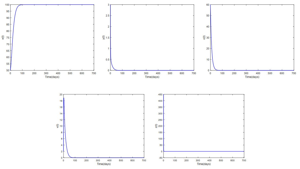
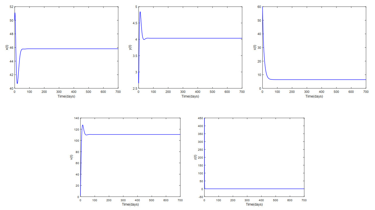
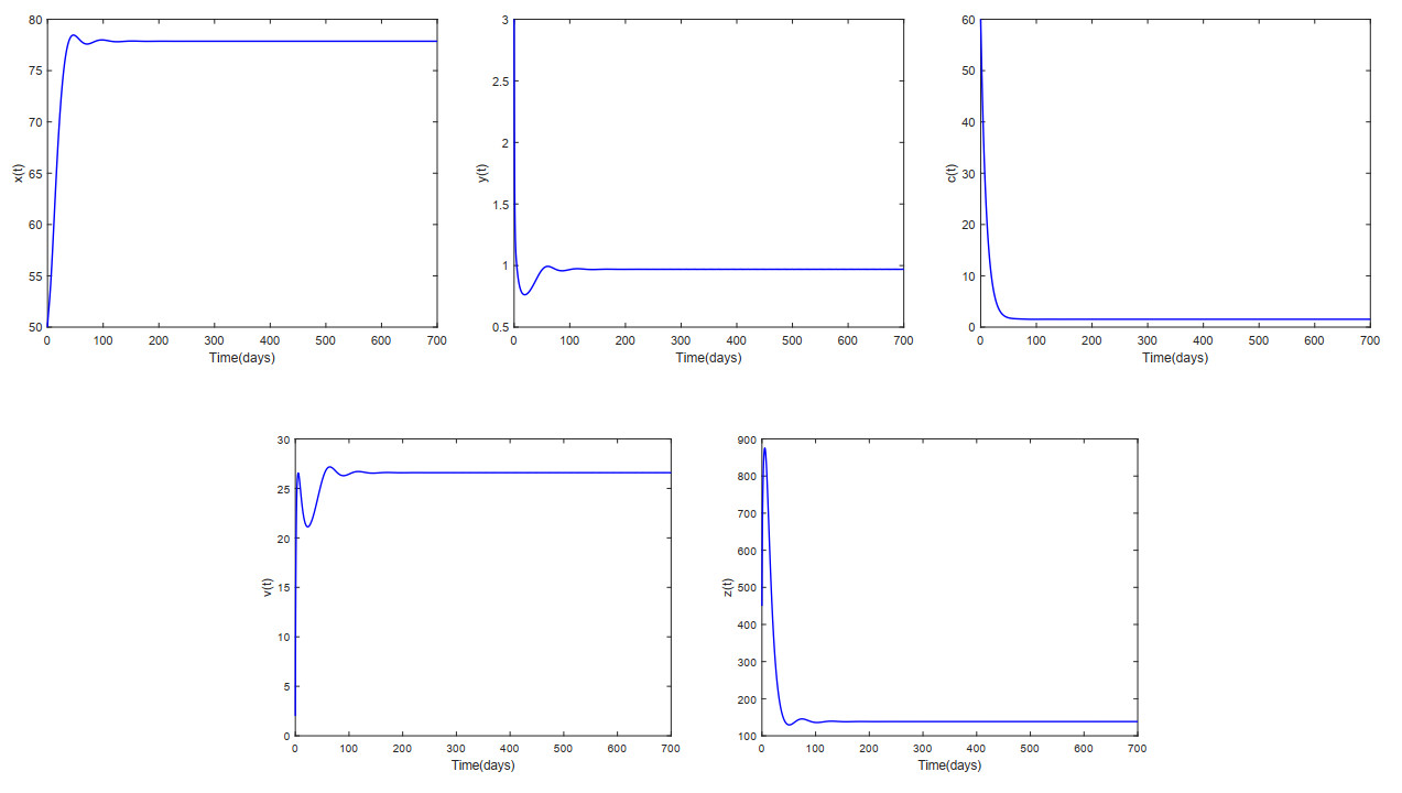
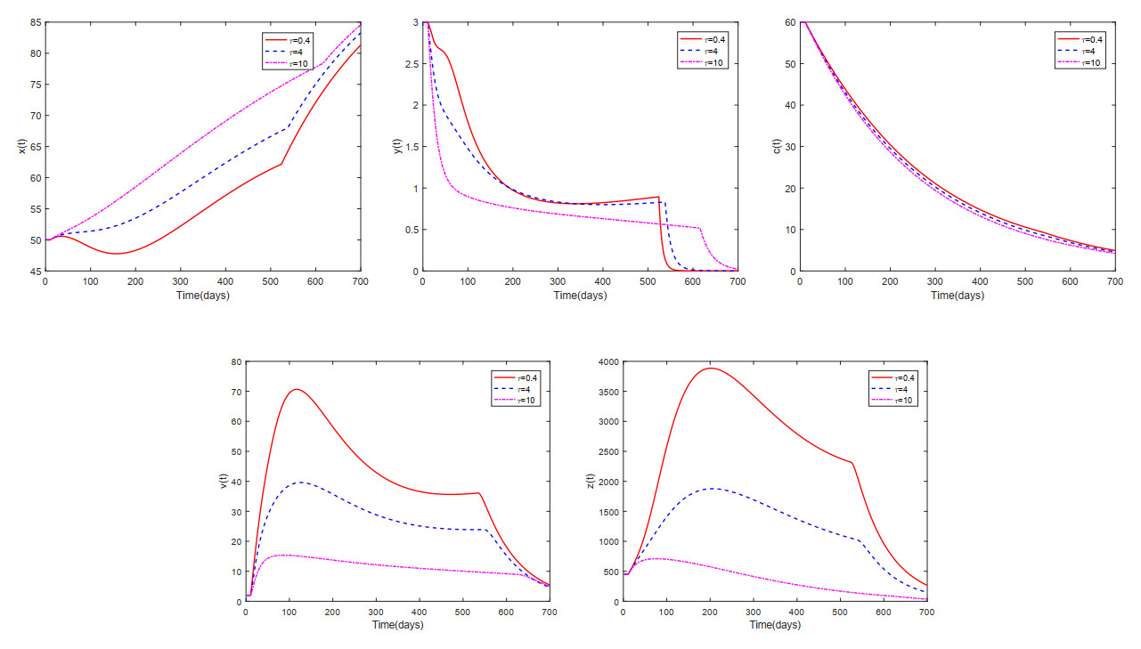
This paper analyzed a cytokine-enhanced viral infection model incorporating three distributed delays: $ (1) $ Intracellular delays in infected $ {\rm CD4}^+ $ T cells induced by inflammatory cytokines and viruses, $ (2) $ delays in $ {\rm CD4}^+ $ T cell activation at inflammatory sites and subsequent cytokine production, and $ (3) $ viral replication delays. By using Lyapunov functionals and LaSalle's invariance principle, we established that each equilibrium exhibits global asymptotic stability under certain conditions. Furthermore, we formulated an optimality system that incorporates delays and then characterized it using Pontryagin's Maximum Principle. Numerical simulations have confirmed the global asymptotic stability of all equilibrium points in the system. Furthermore, for the optimal control system, our simulations not only justified the necessity of incorporating time delay in modeling inflammatory cytokine production but also highlighted the critical importance of tailoring precise HIV treatment strategies according to specific time-delay values.
- inflammatory cytokines,
- pyroptosis,
- distributed delay,
- stability,
- optimal control
Citation: Cuifang Lv, Xiaoyan Chen, Chaoxiong Du. Global dynamics of a cytokine-enhanced viral infection model with distributed delays and optimal control analysis[J]. AIMS Mathematics, 2025, 10(4): 9493-9515. doi: 10.3934/math.2025438

Related Papers:

Abstract

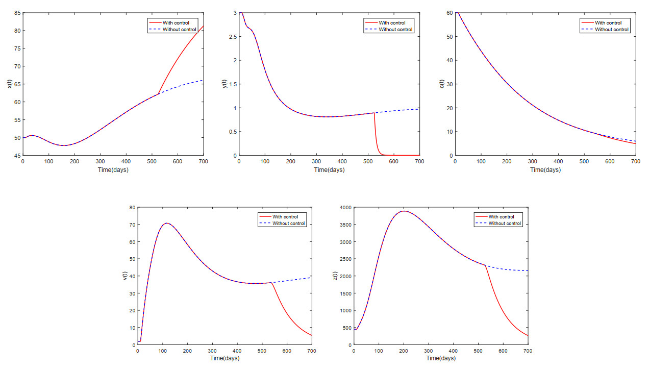
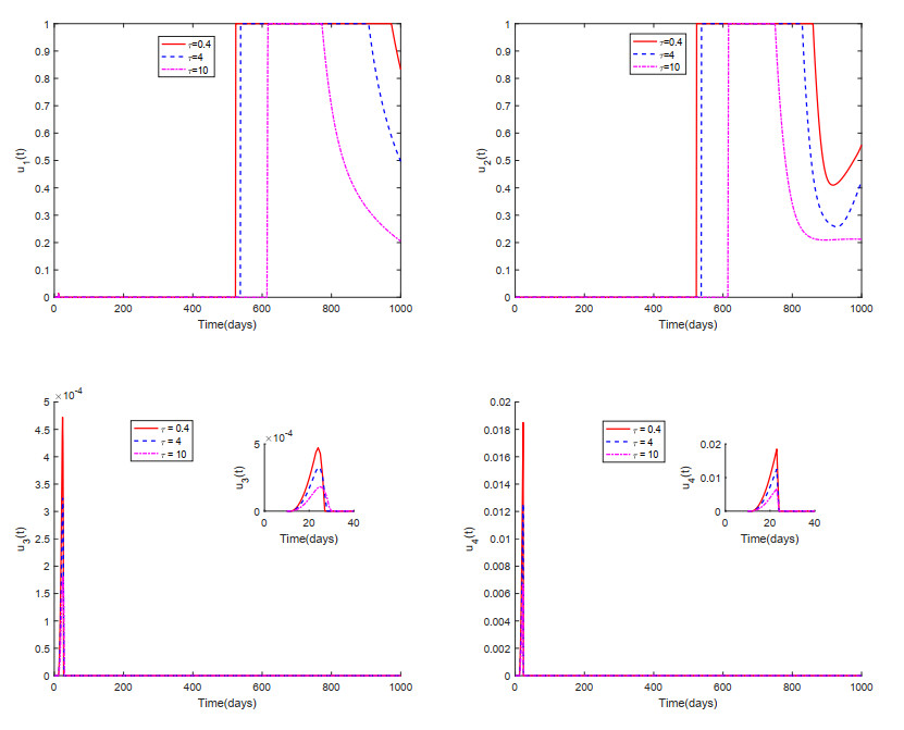
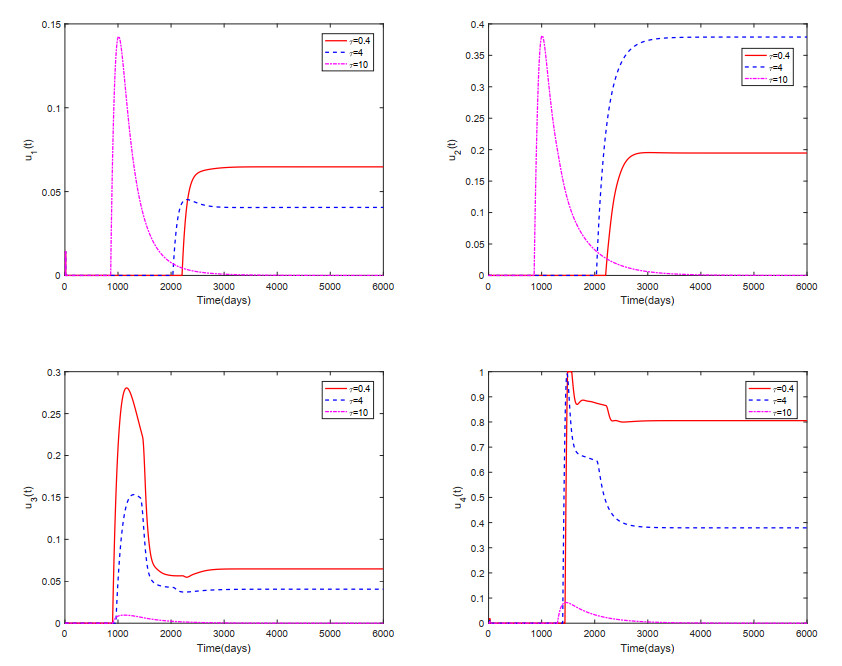
This paper analyzed a cytokine-enhanced viral infection model incorporating three distributed delays: $ (1) $ Intracellular delays in infected $ {\rm CD4}^+ $ T cells induced by inflammatory cytokines and viruses, $ (2) $ delays in $ {\rm CD4}^+ $ T cell activation at inflammatory sites and subsequent cytokine production, and $ (3) $ viral replication delays. By using Lyapunov functionals and LaSalle's invariance principle, we established that each equilibrium exhibits global asymptotic stability under certain conditions. Furthermore, we formulated an optimality system that incorporates delays and then characterized it using Pontryagin's Maximum Principle. Numerical simulations have confirmed the global asymptotic stability of all equilibrium points in the system. Furthermore, for the optimal control system, our simulations not only justified the necessity of incorporating time delay in modeling inflammatory cytokine production but also highlighted the critical importance of tailoring precise HIV treatment strategies according to specific time-delay values.

References

[1]	G. Pantaleo, C. Graziosi, A. S. Fauci, The immuno pathogenesis of human immunodeficiency virus infection, New Engl. J. Med., 328 (1993), 327–335. https://doi.org/10.1056/NEJM199302043280508 doi: 10.1056/NEJM199302043280508
[2]	A. A. Okoye, L. J. Picker, $ {\rm{CD}} 4^+$ T-cell depletion in HIV infection: Mechanisms of immunological failure, Immunol. Rev., 254 (2013), 54–64. https://doi.org/10.1111/imr.12066 doi: 10.1111/imr.12066
[3]	F. V. Atkinsonand, J. R. Haddock, On determining phase spaces for functional differential equations, Funkc. Ekvacioj, 31 (1988), 331–347.
[4]	G. Doitsh, N. Galloway, X. Geng, Z. Y. Yang, K. M. Monroe, O. Zepeda, et al., Pyroptosis drives CD4 T-cell depletion in HIV-1 infection, Nature, 505 (2014), 509–514. https://doi.org/10.1038/nature12940 doi: 10.1038/nature12940
[5]	A. L. Cox, R. F. Siliciano, HIV: Not-so-innocent bystanders, Nature, 505 (2014), 492–493. https://doi.org/10.1038/505492a doi: 10.1038/505492a
[6]	G. Doitsh, M. Cavrois, K. G. Lassen, O. Zepeda, Z. Y. Yang, M. L. Santiago, et al., Abortive HIV infection mediates $ {\rm{CD}} 4^+$ T cell depletion and inflammation in human lymphoid tissue, Cell, 143 (2010), 789–801. https://doi.org/10.1016/j.cell.2010.11.001 doi: 10.1016/j.cell.2010.11.001
[7]	S. P. Wang, P. Hottz, M. Schechter, L. B. Rong, Modeling the slow $ {\rm{CD}} 4^+$ T cell decline in HIV-infected individuals, PLoS. Comput. Biol., 11 (2015), 1004665. https://doi.org/10.1371/journal.pcbi.1004665 doi: 10.1371/journal.pcbi.1004665
[8]	W. Wang, T. Q. Zhang, Caspase-1-mediated pyroptosis of the predominance for driving $ {\rm{CD}} 4^+$ T cells death: A nonlocal spatial mathematical model, B. Math. Biol., 80 (2018), 540–582. https://doi.org/10.1007/s11538-017-0389-8 doi: 10.1007/s11538-017-0389-8
[9]	C. Chen, Y. G. Zhou, Z. J. Ye, Stability and optimal control of a cytokine-enhanced general HIV infection model with antibody immune response and CTLs immune response, Comput. Method. Biomec., 10 (2023), 1–32. https://doi.org/10.1080/10255842.2023.2275248 doi: 10.1080/10255842.2023.2275248
[10]	W. Wang, X. L. Lai, Global stability analysis of a viral infection model in a critical case, Math. Biosci. Eng., 17 (2020), 1442–1449. https://doi.org/10.3934/mbe.2020074 doi: 10.3934/mbe.2020074
[11]	J. H. Xu, Dynamic analysis of a cytokine-enhanced viral infection model with infection age, Math. Biosci. Eng., 20 (2023), 8666–8684. https://doi.org/10.3934/mbe.2023380 doi: 10.3934/mbe.2023380
[12]	M. F. Tan, G. J. Lan, C. J. Wei, Dynamic analysis of HIV infection model with CTL immune response and cell-to-cell transmission, Appl. Math. Lett., 156 (2024), 109140. https://doi.org/10.1016/j.aml.2024.109140 doi: 10.1016/j.aml.2024.109140
[13]	M. A. Alshaikh, N. H. AlShamrani, A. M. Elaiw, Stability of HIV/HTLV co-infection model with effective HIV-specific antibody immune response, Results Phys., 27 (2021), 104448. https://doi.org/10.1016/j.rinp.2021.104448 doi: 10.1016/j.rinp.2021.104448
[14]	Q. Y. Dong, Y. Wang, D. Q. Jiang, Dynamic analysis of an HIV model with CTL immune response and logarithmic Ornstein-Uhlenbeck process, Chaos Soliton. Fract., 191 (2025), 115789. https://doi.org/10.1016/j.chaos.2024.115789 doi: 10.1016/j.chaos.2024.115789
[15]	K. Qi, D. Q. Jiang, T. Hayat, A. Alsaedi, Virus dynamic behavior of a stochastic HIV/AIDS infection model including two kinds of target cell infections and CTL immune responses, Math. Comput. Simulat., 188 (2021), 548–570. https://doi.org/10.1016/j.matcom.2021.05.009 doi: 10.1016/j.matcom.2021.05.009
[16]	Y. Jiang, T. Q. Zhang, Global stability of a cytokine-enhanced viral infection model with nonlinear incidence rate and time delays, Appl. Math. Lett., 132 (2022), 108110. https://doi.org/10.1016/j.aml.2022.108110 doi: 10.1016/j.aml.2022.108110
[17]	T. Q. Zhang, X. N. Xu, X. Z. Wang, Dynamic analysis of a cytokine-enhanced viral infection model with time delays and CTL immune response, Chaos Soliton. Fract., 170 (2023), 113357. https://doi.org/10.1016/j.chaos.2023.113357 doi: 10.1016/j.chaos.2023.113357
[18]	Y. Yang, L. Zou, S. G. Ruan, Global dynamics of a delayed within-host viral infection model with both virus-to-cell and cell-to-cell transmissions, Math. Biosci., 270 (2015), 183–191. https://doi.org/10.1016/j.mbs.2015.05.001 doi: 10.1016/j.mbs.2015.05.001
[19]	P. W. Nelson, A. S. Perelson, Mathematical analysis of delay differential equation models of HIV-1 infection, Math. Biosci., 179 (2002), 73–94. https://doi.org/10.1016/S0025-5564(02)00099-8 doi: 10.1016/S0025-5564(02)00099-8
[20]	R. Xu, Global dynamics of an HIV-1 infection model with distributed intracellular delays, Comput. Math. Appl., 61 (2011), 2799–2805. https://doi.org/10.1016/j.camwa.2011.03.050 doi: 10.1016/j.camwa.2011.03.050
[21]	A. Shohel, R. Sumaiya, M. Kamrujjaman, Optimal treatment strategies to control acute HIV infection, Infect. Dis. Model., 6 (2021), 1202–1219. https://doi.org/10.1016/j.idm.2021.09.004 doi: 10.1016/j.idm.2021.09.004
[22]	J. Danane, K. Allali, Optimal control of an HIV model with CTL cells and latently infected cells, Numer. Algebr. Control, 10 (2020), 207–225. https://doi.org/10.3934/naco.2019048 doi: 10.3934/naco.2019048
[23]	W. Man, A. Xamxinur, Z. D. Teng, Optimal control strategy analysis for an human-animal brucellosis infection model with multiple delays, Heliyon, 8 (2022), e12274. https://doi.org/10.1016/j.heliyon.2022.e12274 doi: 10.1016/j.heliyon.2022.e12274
[24]	H. Khalid, Y. Noura, Optimal control of a delayed HIV infection model with immune response using an efficient numerical method, ISRN Biomath., 11 (2012), 1–7. https://doi.org/10.5402/2012/215124 doi: 10.5402/2012/215124
[25]	H. T. Song, R. F. Wang, S. Q. Liu, Z. Jin, D. H. He, Global stability and optimal control for a COVID-19 model with vaccination and isolation delays, Results Phys., 42 (2022), 106011. https://doi.org/10.1016/j.rinp.2022.106011 doi: 10.1016/j.rinp.2022.106011
[26]	K. Allali, S. Harroudi, Optimal control of an HIV model with a trilinear antibody growth function, Discrete Cont. Dyn.-S, 15 (2022), 501–518. https://doi.org/10.3934/dcdss.2021148 doi: 10.3934/dcdss.2021148
[27]	J. K. Hale, S. M. V. Lunel, Introduction to functional differential equations, Springer Science and Business Media, 1993.
[28]	X. Q. Zhao, The linear stability and basic reproduction numbers for autonomous FDEs, Discrete Cont. Dyn.-S, 17 (2024), 708–719. https://doi.org/10.1016/j.jde.2020.03.027 doi: 10.1016/j.jde.2020.03.027
[29]	C. Zhang, J. W. Song, H. H. Huang, X. Fan, L. Huang, J. N. Deng, et al, NLRP3 inflammasome induces $ {\rm{CD}} 4^+$ T cell loss in chronically HIV-1-Cinfected patients, J. Clin. Invest., 6 (2021), e138861. https://doi.org/10.1172/JCI138861 doi: 10.1172/JCI138861

Reader Comments

Your name:*

Email:*
© 2025 the Author(s), licensee AIMS Press. This is an open access article distributed under the terms of the Creative Commons Attribution License (http://creativecommons.org/licenses/by/4.0)