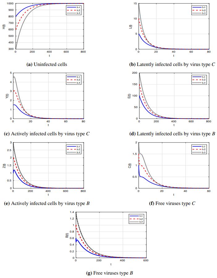
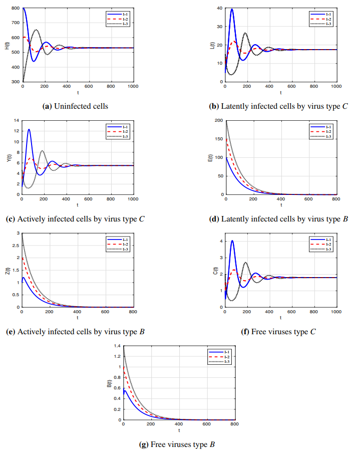
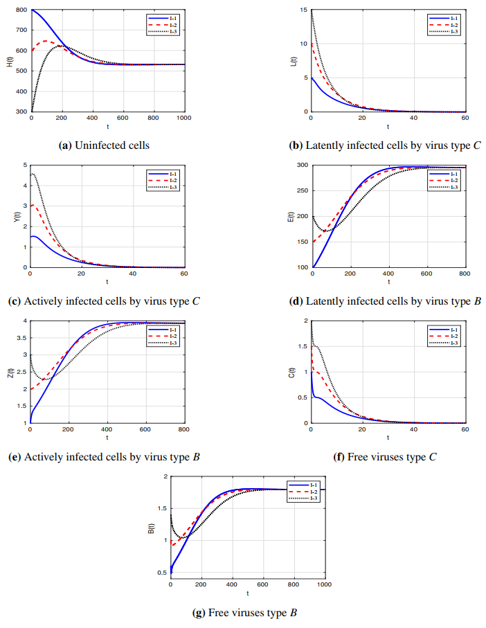
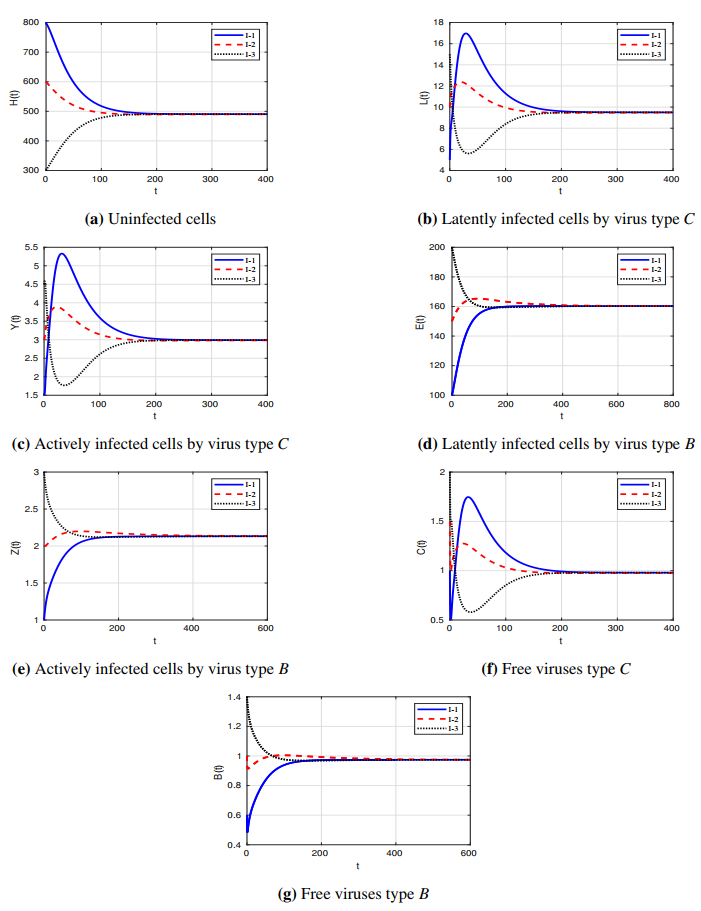
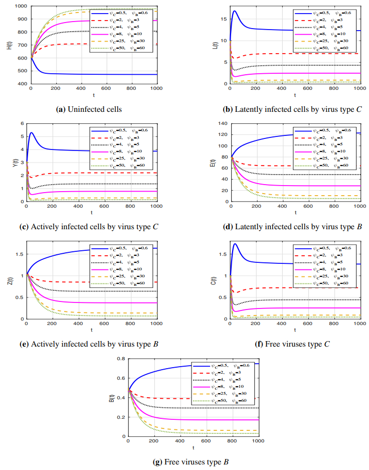
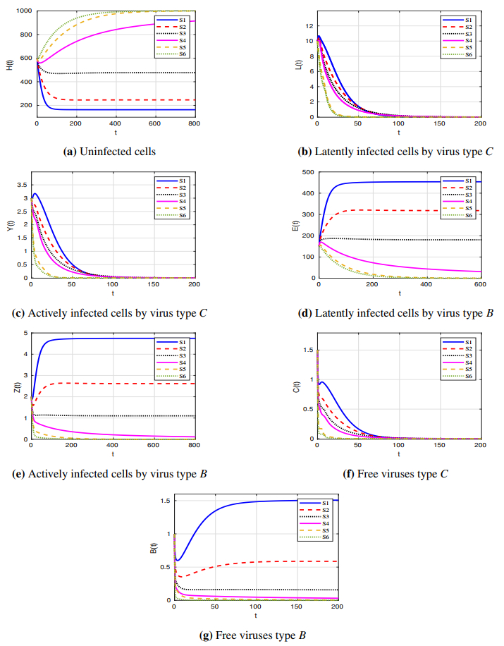
Several mathematical models of two competing viruses (or viral strains) that have been published in the literature assume that the infection rate is determined by bilinear incidence. These models do not show co-existence equilibrium; moreover, they might not be applicable in situations where the virus concentration is high. In this paper, we developed a mathematical model for the co-dynamics of two competing viruses with saturated incidence. The model included the latently infected cells and three types of time delays: discrete (or distributed): (ⅰ) The formation time of latently infected cells; (ⅱ) The activation time of latently infected cells; (ⅲ) The maturation time of newly released virions. We established the mathematical well-posedness and biological acceptability of the model by examining the boundedness and nonnegativity of the solutions. Four equilibrium points were identified, and their stability was examined. Through the application of Lyapunov's approach and LaSalle's invariance principle, we demonstrated the global stability of equilibria. The impact of saturation incidence, latently infected cells, and time delay on the viral co-dynamics was examined. We demonstrated that the saturation could result in persistent viral coinfections. We established conditions under which these types of viruses could coexist. The coexistence conditions were formulated in terms of saturation constants. These findings offered new perspectives on the circumstances under which coexisting viruses (or strains) could live in stable viral populations. It was shown that adding the class of latently infected cells and time delay to the coinfection model reduced the basic reproduction number for each virus type. Therefore, fewer treatment efficacies would be needed to keep the system at the infection-free equilibrium and remove the viral coinfection from the body when utilizing a model with latently infected cells and time delay. To demonstrate the associated mathematical outcomes, numerical simulations were conducted for the model with discrete delays.
Citation: Ahmed M. Elaiw, Ghadeer S. Alsaadi, Aatef D. Hobiny. Global co-dynamics of viral infections with saturated incidence[J]. AIMS Mathematics, 2024, 9(6): 13770-13818. doi: 10.3934/math.2024671
Several mathematical models of two competing viruses (or viral strains) that have been published in the literature assume that the infection rate is determined by bilinear incidence. These models do not show co-existence equilibrium; moreover, they might not be applicable in situations where the virus concentration is high. In this paper, we developed a mathematical model for the co-dynamics of two competing viruses with saturated incidence. The model included the latently infected cells and three types of time delays: discrete (or distributed): (ⅰ) The formation time of latently infected cells; (ⅱ) The activation time of latently infected cells; (ⅲ) The maturation time of newly released virions. We established the mathematical well-posedness and biological acceptability of the model by examining the boundedness and nonnegativity of the solutions. Four equilibrium points were identified, and their stability was examined. Through the application of Lyapunov's approach and LaSalle's invariance principle, we demonstrated the global stability of equilibria. The impact of saturation incidence, latently infected cells, and time delay on the viral co-dynamics was examined. We demonstrated that the saturation could result in persistent viral coinfections. We established conditions under which these types of viruses could coexist. The coexistence conditions were formulated in terms of saturation constants. These findings offered new perspectives on the circumstances under which coexisting viruses (or strains) could live in stable viral populations. It was shown that adding the class of latently infected cells and time delay to the coinfection model reduced the basic reproduction number for each virus type. Therefore, fewer treatment efficacies would be needed to keep the system at the infection-free equilibrium and remove the viral coinfection from the body when utilizing a model with latently infected cells and time delay. To demonstrate the associated mathematical outcomes, numerical simulations were conducted for the model with discrete delays.

| [1] |
L. Lansbury, B. Lim, V. Baskaran, W. S. Lim, Co-infections in people with COVID-19: a systematic review and meta-analysis, J. Infect., 81 (2020), 266–275. https://doi.org/10.1016/j.jinf.2020.05.046 doi: 10.1016/j.jinf.2020.05.046

|
| [2] |
K. Lacombe, J. Rockstroh, HIV and viral hepatitis coinfections: advances and challenges, Gut, 61 (2012), 47–58. https://doi.org/10.1136/gutjnl-2012-302062 doi: 10.1136/gutjnl-2012-302062
|
| [3] |
M. G. Mavilia, G. Y. Wu, HBV-HCV coinfection: viral interactions, management, and viral reactivation, J. Clin. Transl. Hepatol., 6 (2018), 296–305. https://doi.org/10.14218/JCTH.2018.00016 doi: 10.14218/JCTH.2018.00016
|
| [4] | H. O. Hashim, M. K. Mohammed, M. J. Mousa, H. H. Abdulameer, A. T. Alhassnawi, S. A. Hassan, et al., Infection with different strains of SARS-CoV-2 in patients with COVID-19, Arch. Biol. Sci., 72 (2020), 575–585. |
| [5] |
S. Shoraka, S. R. Mohebbi, S. M. Hosseini, A. Ghaemi, M. R. Zali, SARS-CoV-2 and chronic hepatitis B: focusing on the possible consequences of co-infection, J. Clin. Virol. Plus, 3 (2023), 100167. https://doi.org/10.1016/j.jcvp.2023.100167 doi: 10.1016/j.jcvp.2023.100167
|
| [6] |
M. A. Nowak, C. R. M. Bangham, Population dynamics of immune responses to persistent viruses, Science, 272 (1996), 74–79. https://doi.org/10.1126/science.272.5258.74 doi: 10.1126/science.272.5258.74
|
| [7] |
P. de Leenheer, S. S. Pilyugin, Multistrain virus dynamics with mutations: a global analysis, Math. Med. Biol., 25 (2008), 285–322. https://doi.org/10.1093/imammb/dqn023 doi: 10.1093/imammb/dqn023
|
| [8] |
L. Pinky, H. M. Dobrovolny, SARS-CoV-2 coinfections: could influenza and the common cold be beneficial? J. Med. Virol., 92 (2020), 2623–2630. https://doi.org/10.1002/jmv.26098 doi: 10.1002/jmv.26098
|
| [9] |
M. D. Nowak, E. M. Sordillo, M. R. Gitman, A. E. P. Mondolfi, Coinfection in SARS-CoV-2 infected patients: where are influenza virus and rhinovirus/enterovirus? J. Med. Virol., 92 (2020), 1699–1700. https://doi.org/10.1002/jmv.25953 doi: 10.1002/jmv.25953
|
| [10] |
S. Kalinichenko, D. Komkov, D. Mazurov, HIV-1 and HTLV-1 transmission modes: mechanisms and importance for virus spread, Viruses, 14 (2022), 152. https://doi.org/10.3390/v14010152 doi: 10.3390/v14010152
|
| [11] |
J. Schmidt, H. E. Blum, R. Thimme, T-cell responses in hepatitis B and C virus infection: similarities and differences, Emerg. Micro. Infect., 2 (2013), e15. https://doi.org/10.1038/emi.2013.14 doi: 10.1038/emi.2013.14
|
| [12] |
M. Ruiz Silva, J. A. A. Briseño, V. Upasani, H. van der Ende-Metselaar, J. M. Smit, I. A. Rodenhuis-Zybert, Suppression of chikungunya virus replication and differential innate responses of human peripheral blood mononuclear cells during co-infection with dengue virus, PLoS Negl. Trop. Dis., 11 (2017), e0005712. https://doi.org/10.1371/journal.pntd.0005712 doi: 10.1371/journal.pntd.0005712
|
| [13] |
A. Nurtay, M. G. Hennessy, J. Sardanyés, L. Alsedà, S. F. Elena, Theoretical conditions for the coexistence of viral strains with differences in phenotypic traits: a bifurcation analysis, R. Soc. Open Sci., 6 (2019), 181179. https://doi.org/10.1098/rsos.181179 doi: 10.1098/rsos.181179
|
| [14] |
P. J. Goulder, B. D. Walker, HIV-1 superinfection: a word of caution, New Engl. J. Med., 347 (2002), 756–758. https://doi.org/10.1056/NEJMe020091 doi: 10.1056/NEJMe020091
|
| [15] |
Y. He, W. Ma, S. Dang, L. Chen, R. Zhang, S. Mei, et al., Possible recombination between two variants of concern in a COVID-19 patient, Emerg. Micro. Infect., 11 (2022), 552–555. https://doi.org/10.1080/22221751.2022.2032375 doi: 10.1080/22221751.2022.2032375
|
| [16] |
A. M. Elaiw, N. H. AlShamrani, Analysis of a within-host HIV/HTLV-I co-infection model with immunity, Virus Res., 295 (2021), 198204. https://doi.org/10.1016/j.virusres.2020.198204 doi: 10.1016/j.virusres.2020.198204
|
| [17] |
A. M. Elaiw, R. S. Alsulami, A. D. Hobiny, Modeling and stability analysis of within-host IAV/SARS-CoV-2 coinfection with antibody immunity, Mathematics, 10 (2022), 4382. https://doi.org/10.3390/math10224382 doi: 10.3390/math10224382
|
| [18] |
A. M. Elaiw, A. S. Shflot, A. D. Hobiny, Global stability of delayed SARS-CoV-2 and HTLV-I coinfection models within a host, Mathematics, 10 (2022), 4756. https://doi.org/10.3390/math10244756 doi: 10.3390/math10244756
|
| [19] |
A. M. Elaiw, A. D. Al Agha, S. A. Azoz, E. Ramadan, Global analysis of within-host SARS-CoV-2/HIV coinfection model with latency, Eur. Phys. J. Plus, 137 (2022), 174. https://doi.org/10.1140/epjp/s13360-022-02387-2 doi: 10.1140/epjp/s13360-022-02387-2
|
| [20] |
H. Nampala, S. Livingstone, L. Luboobi, J. Y. T. Mugisha, C. Obua, M. Jablonska-Sabuka, Modelling hepatotoxicity and antiretroviral therapeutic effect in HIV/HBV coinfection, Math. Biosci., 302 (2018), 67–79. https://doi.org/10.1016/j.mbs.2018.05.012 doi: 10.1016/j.mbs.2018.05.012
|
| [21] |
R. Birger, R. Kouyos, J. Dushoff, B. Grenfell, Modeling the effect of HIV coinfection on clearance and sustained virologic response during treatment for hepatitis C virus, Epidemics, 12 (2015), 1–10. https://doi.org/10.1016/j.epidem.2015.04.001 doi: 10.1016/j.epidem.2015.04.001
|
| [22] |
L. Rong, Z. Feng, A. S. Perelson, Emergence of HIV-1 drug resistance during antiretroviral treatment, Bull. Math. Biol., 69 (2007), 2027–2060. https://doi.org/10.1007/s11538-007-9203-3 doi: 10.1007/s11538-007-9203-3
|
| [23] |
P. Wu, H. Zhao, Dynamics of an HIV infection model with two infection routes and evolutionary competition between two viral strains, Appl. Math. Modell., 84 (2020), 240–264. https://doi.org/10.1016/j.apm.2020.03.040 doi: 10.1016/j.apm.2020.03.040
|
| [24] |
B. J. Nath, K. Sadri, H. K. Sarmah, K. Hosseini, An optimal combination of antiretroviral treatment and immunotherapy for controlling HIV infection, Math. Comput. Simul., 217 (2024), 226–243. https://doi.org/10.1016/j.matcom.2023.10.012 doi: 10.1016/j.matcom.2023.10.012
|
| [25] |
Y. Liu, Y. Wang, D. Jiang, Dynamic behaviors of a stochastic virus infection model with Beddington-DeAngelis incidence function, eclipse-stage and Ornstein-Uhlenbeck process, Math. Biosci., 2024 (2024), 109154. https://doi.org/10.1016/j.mbs.2024.109154 doi: 10.1016/j.mbs.2024.109154
|
| [26] |
O. Lambotte, M. L. Chaix, B. Gubler, N. Nasreddine, C. Wallon, C. Goujard, et al., The lymphocyte HIV reservoir in patients on long-term HAART is a memory of virus evolution, AIDS, 18 (2004), 1147–1158. https://doi.org/10.1097/00002030-200405210-00008 doi: 10.1097/00002030-200405210-00008
|
| [27] |
W. Chen, Z. Teng, L. Zhang, Global dynamics for a drug-sensitive and drug-resistant mixed strains of HIV infection model with saturated incidence and distributed delays, Appl. Math. Comput., 406 (2021), 126284. https://doi.org/10.1016/j.amc.2021.126284 doi: 10.1016/j.amc.2021.126284
|
| [28] |
A. Perelson, A. Neumann, M. Markowitz, J. Leonard, D. Ho, HIV-1 dynamics in vivo: virion clearance rate, infected cell life-span, and viral generation time, Science, 271 (1996), 1582–1586. https://doi.org/10.1126/science.271.5255.1582 doi: 10.1126/science.271.5255.1582
|
| [29] |
R. V. Culshaw, S. Ruan, A delay-differential equation model of HIV infection of CD4$^{+}$ T-cells, Math. Biosci., 165 (2000), 27–39. https://doi.org/10.1016/s0025-5564(00)00006-7 doi: 10.1016/s0025-5564(00)00006-7
|
| [30] |
S. K. Sahani, Yashi, Effects of eclipse phase and delay on the dynamics of HIV infection, J. Biol. Syst., 26 (2018), 421–454. https://doi.org/10.1142/S0218339018500195 doi: 10.1142/S0218339018500195
|
| [31] |
R. Xu, Global dynamics of an HIV-1 infection model with distributed intracellular delays, Comput. Math. Appl., 61 (2011), 2799–2805. https://doi.org/10.1016/j.camwa.2011.03.050 doi: 10.1016/j.camwa.2011.03.050
|
| [32] |
J. Li, X. Wang, Y. Chen, Analysis of an age-structured HIV infection model with cell-to-cell transmission, Eur. Phys. J. Plus, 139 (2024), 78. https://doi.org/10.1140/epjp/s13360-024-04873-1 doi: 10.1140/epjp/s13360-024-04873-1
|
| [33] |
D. Ebert, C. D. Zschokke-Rohringer, H. J. Carius, Dose effects and density-dependent regulation of two microparasites of Daphnia magna, Oecologia, 122 (2000), 200–209. https://doi.org/10.1007/PL00008847 doi: 10.1007/PL00008847
|
| [34] |
X. Song, A. U. Neumann, Global stability and periodic solution of the viral dynamics, J. Math. Anal. Appl., 329 (2007), 281–297. https://doi.org/10.1016/j.jmaa.2006.06.064 doi: 10.1016/j.jmaa.2006.06.064
|
| [35] |
O. A. Razzaq, N. A. Khan, M. Faizan, A. Ara, S. Ullah, Behavioral response of population on transmissibility and saturation incidence of deadly pandemic through fractional order dynamical system, Results Phys., 26 (2021), 104438. https://doi.org/10.1016/j.rinp.2021.104438 doi: 10.1016/j.rinp.2021.104438
|
| [36] |
W. Chen, N. Tuerxun, Z. Teng, The global dynamics in a wild-type and drug-resistant HIV infection model with saturated incidence, Adv. Differ. Equations, 2020 (2020), 25. https://doi.org/10.1186/s13662-020-2497-2 doi: 10.1186/s13662-020-2497-2
|
| [37] | W. Chen, L. Zhang, N. Wang, Z. Teng, Bifurcation analysis and chaos for a double-strains HIV coinfection model with intracellular delays, saturated incidence and logistic growth, Saturated Incidence Logist. Growth, 2023. https://doi.org/10.21203/rs.3.rs-3132841/v1 |
| [38] |
T. Li, Y. Guo, Modeling and optimal control of mutated COVID-19 (Delta strain) with imperfect vaccination, Chaos Solitons Fract., 156 (2022), 111825. https://doi.org/10.1016/j.chaos.2022.111825 doi: 10.1016/j.chaos.2022.111825
|
| [39] |
Y. Guo, T. Li, Modeling the competitive transmission of the Omicron strain and Delta strain of COVID-19, J. Math. Anal. Appl., 526 (2023), 127283. https://doi.org/10.1016/j.jmaa.2023.127283 doi: 10.1016/j.jmaa.2023.127283
|
| [40] | J. K. Hale, S. M. V. Lunel, Introduction to functional differential equations, Springer-Verlag, 1993. |
| [41] | Y. Kuang, Delay differential equations with applications in population dynamics, Academic Press, 1993. |
| [42] |
D. Wodarz, D. C. Krakauer, Defining CTL-induced pathology: implications for HIV, Virology, 274 (2000), 94–104. https://doi.org/10.1006/viro.2000.0399 doi: 10.1006/viro.2000.0399
|
| [43] | A. S. Perelson, Modeling the interaction of the immune system with HIV, In: C. Castillo-Chavez, Mathematical and statistical approaches to AIDS epidemiology, Springer Berlin Heidelberg, 1989,350–370. https://doi.org/10.1007/978-3-642-93454-4_17 |
| [44] | A. S. Perelson, D. E. Kirschner, R. de Boer, Dynamics of HIV Infection of CD4$^{+}$ T cells, Math. Biosci., 114 (1993), 81–125. |
| [45] |
W. A. Woldegerima, M. I. Teboh-Ewungkem, G. A. Ngwa, The impact of recruitment on the dynamics of an immune-suppressed within-human-host model of the Plasmodium falciparum parasite, Bull. Math. Biol., 81 (2019), 4564–4619. https://doi.org/10.1007/s11538-018-0436-0 doi: 10.1007/s11538-018-0436-0
|
| [46] |
P. van den Driessche, J. Watmough, Reproduction numbers and sub-threshold endemic equilibria for compartmental models of disease transmission, Math. Biosci., 180 (2002), 29–48. https://doi.org/10.1016/s0025-5564(02)00108-6 doi: 10.1016/s0025-5564(02)00108-6
|
| [47] |
A. Korobeinikov, Global properties of basic virus dynamics models, Bull. Math. Biol., 66 (2004), 879–883. https://doi.org/10.1016/j.bulm.2004.02.001 doi: 10.1016/j.bulm.2004.02.001
|
| [48] | H. K. Khalil, Nonlinear systems, 3 Eds., Prentice Hall, 2002. |
| [49] |
L. Pinky, G. González-Parran, H. M. Dobrovolny, Superinfection and cell regeneration can lead to chronic viral coinfections, J. Theor. Biol., 466 (2019), 24–38. https://doi.org/10.1016/j.jtbi.2019.01.011 doi: 10.1016/j.jtbi.2019.01.011
|
| [50] |
F. Li, W. Ma, Dynamics analysis of an HTLV-1 infection model with mitotic division of actively infected cells and delayed CTL immune response, Math. Methods Appl. Sci., 41 (2018), 3000–3017. https://doi.org/10.1002/mma.4797 doi: 10.1002/mma.4797
|
| [51] |
N. H. Alshamrani, Stability of an HTLV-HIV coinfection model with multiple delays and CTL-mediated immunity, Adv. Differ. Equations, 2021 (2021), 270. https://doi.org/10.1186/s13662-021-03416-7 doi: 10.1186/s13662-021-03416-7
|
| [52] |
D. S. Callaway, A. S. Perelson, HIV-1 infection and low steady state viral loads, Bull. Math. Biol., 64 (2002), 29–64. https://doi.org/10.1006/bulm.2001.0266 doi: 10.1006/bulm.2001.0266
|
| [53] |
Y. Wang, J. Liu, L. Liu, Viral dynamics of an HIV model with latent infection incorporating antiretroviral therapy, Adv. Differ. Equations, 2016 (2016), 225. https://doi.org/10.1186/s13662-016-0952-x doi: 10.1186/s13662-016-0952-x
|
| [54] |
Y. Wang, J. Liu, J. M. Heffernan, Viral dynamics of an HTLV-I infection model with intracellular delay and CTL immune response delay, J. Math. Anal. Appl., 459 (2018), 506–527. https://doi.org/10.1016/j.jmaa.2017.10.027 doi: 10.1016/j.jmaa.2017.10.027
|
| [55] |
B. Asquith, C. R. Bangham, Quantifying HTLV-I dynamics, Immunol. Cell Biol., 85 (2007), 280–286. https://doi.org/10.1038/sj.icb.7100050 doi: 10.1038/sj.icb.7100050
|
| [56] |
G. Huang, W. Ma, Y. Takeuchi, Global properties for virus dynamics model with Beddington-DeAngelis functional response, Appl. Math. Lett., 22 (2009), 1690–1693. https://doi.org/10.1016/j.aml.2009.06.004 doi: 10.1016/j.aml.2009.06.004
|
| [57] |
X. Zhou, J. Cui, Global stability of the viral dynamics with Crowley-Martin functional response, Bull. Korean Math. Soc., 48 (2011), 555–574. https://doi.org/10.4134/BKMS.2011.48.3.555 doi: 10.4134/BKMS.2011.48.3.555
|
| [58] |
K. Hattaf, N. Yousfi, A class of delayed viral infection models with general incidence rate and adaptive immune response, Int. J. Dyn. Control, 4 (2016), 254–265. https://doi.org/10.1007/s40435-015-0158-1 doi: 10.1007/s40435-015-0158-1
|
| [59] |
G. Huang, Y. Takeuchi, W. Ma, Lyapunov functionals for delay differential equations model of viral infections, SIAM J. Appl. Math., 70 (2010), 2693–2708. https://doi.org/10.1137/090780821 doi: 10.1137/090780821
|
| [60] |
K. Hattaf, A new mixed fractional derivative with applications in computational biology, Computation, 12 (2024), 7. https://doi.org/10.3390/computation12010007 doi: 10.3390/computation12010007
|
| [61] |
J. Danane, K. Allali, Z. Hammouch, Mathematical analysis of a fractional differential model of HBV infection with antibody immune response, Chaos Solitons Fract., 136 (2020), 109787. https://doi.org/10.1016/j.chaos.2020.109787 doi: 10.1016/j.chaos.2020.109787
|
| [62] |
Y. Guo, T. Li, Fractional-order modeling and optimal control of a new online game addiction model based on real data, Commun. Nonlinear Sci. Numer. Simul., 121 (2023), 107221. https://doi.org/10.1016/j.cnsns.2023.107221 doi: 10.1016/j.cnsns.2023.107221
|
| [63] |
W. Adel, H. Günerhan, K. S. Nisar, P. Agarwal, A. El-Mesady, Designing a novel fractional order mathematical model for COVID-19 incorporating lockdown measures, Sci. Rep., 14 (2024), 2926. https://doi.org/10.1038/s41598-023-50889-5 doi: 10.1038/s41598-023-50889-5
|
| [64] |
N. Bellomo, D. Burini, N. Outada, Multiscale models of COVID-19 with mutations and variants, Networks Heterog. Media, 17 (2022), 293–310. https://doi.org/10.3934/nhm.2022008 doi: 10.3934/nhm.2022008
|
| [65] |
D. Burini, D. Knopoff, Epidemics and society-a multiscale vision from the small world to the globally interconnected world, Math. Models Methods Appl. Sci., 34 (2024), 295. https://doi.org/10.1142/S0218202524500295 doi: 10.1142/S0218202524500295
|
Figures(6) / Tables(4)

Ahmed M. Elaiw, Ghadeer S. Alsaadi, Aatef D. Hobiny. Global co-dynamics of viral infections with saturated incidence[J]. AIMS Mathematics, 2024, 9(6): 13770-13818. doi: 10.3934/math.2024671


 DownLoad: