Count data modeling and its practical applications have garnered significant attention in recent research, owing to its relevance in a wide range of fields. This study specifically explores a novel discrete distribution characterized by two parameters, which is derived using the survival discretization method. The statistical properties of this distribution are thoroughly explained in closed forms, with several key mathematical attributes also derived. These characteristics underscore the distribution's effectiveness in modeling data that exhibit (right-skewed) asymmetry and have extended heavy tails, making it particularly suitable for such real-world applications. Furthermore, the failure rate function corresponding to this distribution is particularly appropriate for scenarios characterized by an increasing or bathtub-shaped failure rate over time. The model is also highly versatile, offering valuable insights into probabilistic modeling for datasets that display over dispersion, under dispersion, or equi dispersion. The study introduces several estimation techniques, including the maximum product of spacings, Anderson–Darling, right–tail Anderson–Darling, maximum likelihood estimation, least squares, weighted least squares, Cramer–Von–Mises, and percentile methods. Each of these methods is explained in detail, providing a comprehensive understanding of their application. A ranking simulation study is conducted to evaluate the performance of these estimators across varying sample sizes, using ranking techniques to identify the most effective estimator in different scenarios. The analysis of real-world datasets from biotechnology and industrial engineering further demonstrates the practical utility and relevance of the proposed model. The results highlight the model's ability to offer accurate and insightful analyses, reinforcing its significance in count data modeling and its wide-ranging applications.
Citation: Mohamed S. Algolam, Mohamed S. Eliwa, Mohamed El-Dawoody, Mahmoud El-Morshedy. A discrete extension of the Xgamma random variable: mathematical framework, estimation methods, simulation ranking, and applications to radiation biology and industrial engineering data[J]. AIMS Mathematics, 2025, 10(3): 6069-6101. doi: 10.3934/math.2025277
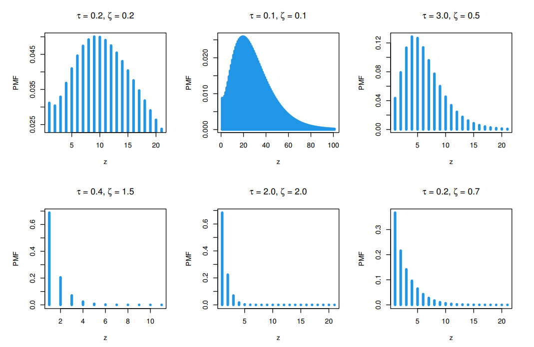
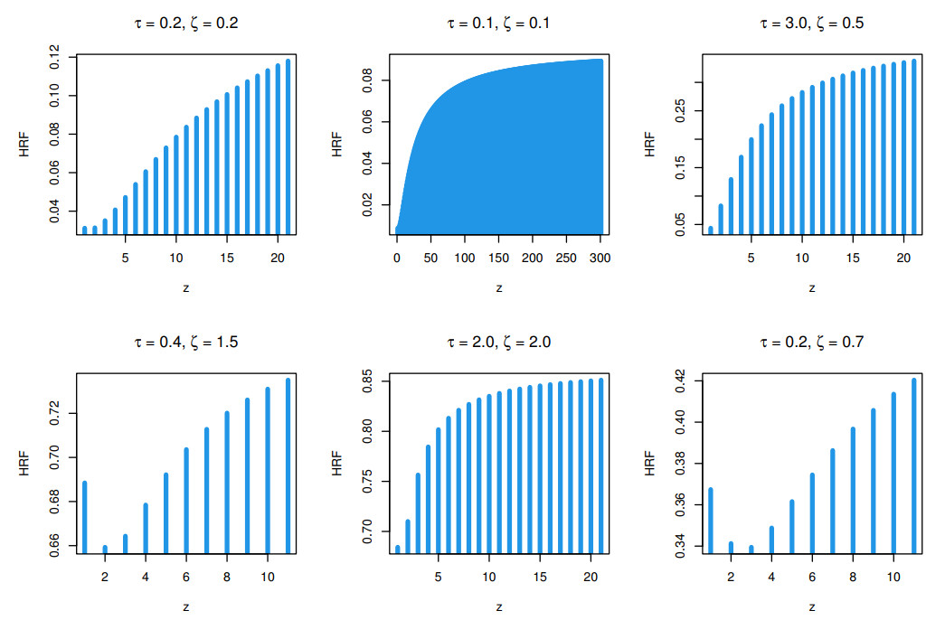
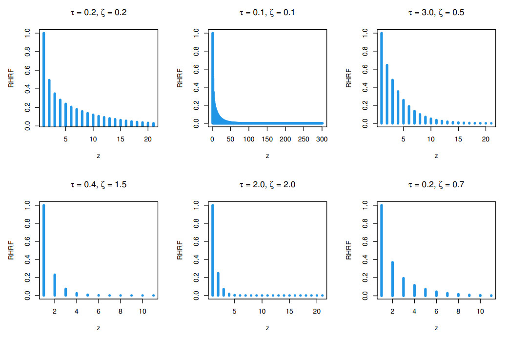
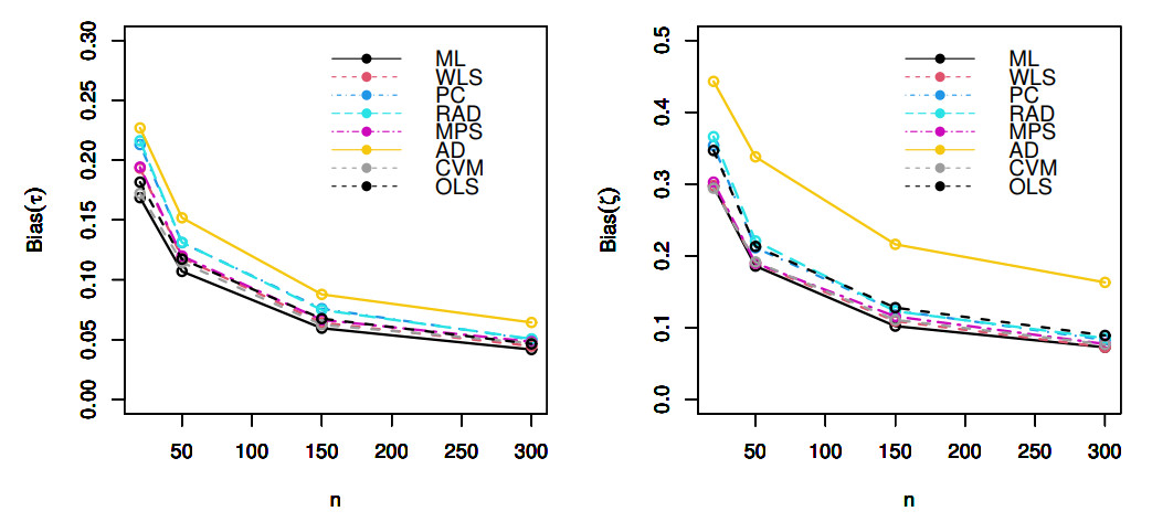
Count data modeling and its practical applications have garnered significant attention in recent research, owing to its relevance in a wide range of fields. This study specifically explores a novel discrete distribution characterized by two parameters, which is derived using the survival discretization method. The statistical properties of this distribution are thoroughly explained in closed forms, with several key mathematical attributes also derived. These characteristics underscore the distribution's effectiveness in modeling data that exhibit (right-skewed) asymmetry and have extended heavy tails, making it particularly suitable for such real-world applications. Furthermore, the failure rate function corresponding to this distribution is particularly appropriate for scenarios characterized by an increasing or bathtub-shaped failure rate over time. The model is also highly versatile, offering valuable insights into probabilistic modeling for datasets that display over dispersion, under dispersion, or equi dispersion. The study introduces several estimation techniques, including the maximum product of spacings, Anderson–Darling, right–tail Anderson–Darling, maximum likelihood estimation, least squares, weighted least squares, Cramer–Von–Mises, and percentile methods. Each of these methods is explained in detail, providing a comprehensive understanding of their application. A ranking simulation study is conducted to evaluate the performance of these estimators across varying sample sizes, using ranking techniques to identify the most effective estimator in different scenarios. The analysis of real-world datasets from biotechnology and industrial engineering further demonstrates the practical utility and relevance of the proposed model. The results highlight the model's ability to offer accurate and insightful analyses, reinforcing its significance in count data modeling and its wide-ranging applications.

| [1] |
J. Melnikow, A. Padovani, M. Miller, Frontline physician burnout during the COVID-19 pandemic: national survey findings, BMC Health Serv. Res., 22 (2022), 365. https://doi.org/10.1186/s12913-022-07728-6 doi: 10.1186/s12913-022-07728-6

|
| [2] |
J. Mapes, Using big data to study small places: small-town voting patterns in the 2020 US presidential election, Growth Change, 55 (2024), e12730. https://doi.org/10.1111/grow.12730 doi: 10.1111/grow.12730
|
| [3] |
E. Clough, T. Barrett, S. E. Wilhite, P. Ledoux, C. Evangelista, I. F. Kim, et al., NCBI GEO: archive for gene expression and epigenomics data sets: 23-year update, Nucleic Acids Res., 52 (2024), D138–D144. https://doi.org/10.1093/nar/gkad965 doi: 10.1093/nar/gkad965
|
| [4] |
S. Yang, D. Meng, A. Díaz, H. Yang, X. Su, A. M. D. Jesus, Probabilistic modeling of uncertainties in reliability analysis of mid-and high-strength steel pipelines under hydrogen-induced damage, Int. J. Struct. Integr., 16 (2025), 39–59. https://doi.org/10.1108/IJSI-10-2024-0177 doi: 10.1108/IJSI-10-2024-0177
|
| [5] | S. Yang, D. Meng, H. Yang, C. Luo, X. Su, Enhanced soft Monte Carlo simulation coupled with support vector regression for structural reliability analysis, In: Proceedings of the Institution of Civil Engineers-Transport, Emerald Publishing Limited, 2024, 1–16. https://doi.org/10.1680/jtran.24.00128 |
| [6] |
D. Meng, H. Yang, S. Yang, Y. Zhang, A. M. De Jesus, J. Correia, et al., Kriging-assisted hybrid reliability design and optimization of offshore wind turbine support structure based on a portfolio allocation strategy, Ocean Eng., 295 (2024), 116842. https://doi.org/10.1016/j.oceaneng.2024.116842 doi: 10.1016/j.oceaneng.2024.116842
|
| [7] | S. Sen, S. K. Ghosh, H. Al-Mofleh, The Mirra distribution for modeling time-to-event data sets, In: Dtrategic management, decision theory, and decision science: contributions to policy issues, Singapore: Springer, 2021. https://doi.org/10.1007/978-981-16-1368-5_5 |
| [8] |
D. Roy, Discrete Rayleigh distribution, IEEE Trans. Reliab., 53 (2004), 255–260. https://doi.org/10.1109/TR.2004.829161 doi: 10.1109/TR.2004.829161
|
| [9] |
M. El-Morshedy, M. S. Eliwa, E. Altun, Discrete Burr-Hatke distribution with properties, estimation methods and regression model, IEEE Access, 8 (2020), 74359–74370. https://doi.org/10.1109/ACCESS.2020.2988431 doi: 10.1109/ACCESS.2020.2988431
|
| [10] |
H. Krishna, P. S. Pundir, Discrete Burr and discrete Pareto distributions, Stat. Methodol., 6 (2009), 177–188. https://doi.org/10.1016/j.stamet.2008.07.001 doi: 10.1016/j.stamet.2008.07.001
|
| [11] | T. Hussain, M. Ahmad, Discrete inverse Rayleigh distribution, Pakistan J. Stat., 30 (2014). |
| [12] | A. E. Abd EL-Hady, M. A. Hegazy, A. A. EL-Helbawy, A discrete exponentiated generalized family of distributions, Comput. J. Math. Stat. Sci., 2 (2023), 303–327. |
| [13] | A. R. E. Alosey, A. M. Gemeay, A novel version of geometric distribution: method and application, Comput. J. Math. Stat. Scie., 4 (2025), 1–16. |
| [14] |
M. A. Jazi, C. D. Lai, M. H. Alamatsaz, A discrete inverse Weibull distribution and estimation of its parameters, Stat. Methodol., 7 (2010), 121–132. https://doi.org/10.1016/j.stamet.2009.11.001 doi: 10.1016/j.stamet.2009.11.001
|
| [15] |
E. Gómez-Déniz, E. Calderín-Ojeda, The discrete Lindley distribution: properties and applications, J. Stat. Comput. Simul., 81 (2011), 1405–1416. https://doi.org/10.1080/00949655.2010.487825 doi: 10.1080/00949655.2010.487825
|
| [16] |
J. M. Jia, Z. Z. Yan, X. Y. Peng, A new discrete extended Weibull distribution, IEEE Access, 7 (2019), 175474–175486. https://doi.org/10.1109/ACCESS.2019.2957788 doi: 10.1109/ACCESS.2019.2957788
|
| [17] |
E. Altun, A new generalization of geometric distribution with properties and applications, Commun. Stat.-Simul. Comput., 49 (2020), 793–807. https://doi.org/10.1080/03610918.2019.1639739 doi: 10.1080/03610918.2019.1639739
|
| [18] |
E. Gómez-Déniz, Another generalization of the geometric distribution, Test, 19 (2010), 399–415. https://doi.org/10.1007/s11749-009-0169-3 doi: 10.1007/s11749-009-0169-3
|
| [19] | M. A. Hegazy, R. E. Abd El-Kader, A. A. El-Helbawy, G. R. Al-Dayian, Bayesian estimation and prediction of discrete Gompertz distribution, J. Adv. Math. Comput. Sci., 36 (2021), 1–21. |
| [20] |
V. Nekoukhou, M. H. Alamatsaz, H. Bidram, Discrete generalized exponential distribution of a second type, Statistics, 47 (2013), 876–887. https://doi.org/10.1080/02331888.2011.633707 doi: 10.1080/02331888.2011.633707
|
| [21] |
A. S. Eldeeb, M. Ahsan-ul-Haq, M. S. Eliwa, A discrete Ramos-Louzada distribution for asymmetric and over-dispersed data with leptokurtic-shaped: properties and various estimation techniques with inference, AIMS Math., 7 (2022), 1726–1741. https://doi.org/10.3934/math.2022099 doi: 10.3934/math.2022099
|
| [22] | T. Hussain, M. Aslam, M. Ahmad, A two parameter discrete Lindley distribution, Rev. Colomb. Estad., 39 (2016), 45–61. |
| [23] | B. C. Arnold, N. Balakrishnan, H. N. Nagaraja, A first course in order statistics, Society for Industrial and Applied Mathematics, 2008. |
| [24] |
R. Shanker, H. Fesshaye, On Poisson-Sujatha distribution and its applications to model count data from biological sciences, Biometrics Biostat. Int. J., 3 (2016), 1–7. https://doi.org/10.15406/bbij.2015.02.00036 doi: 10.15406/bbij.2015.02.00036
|
| [25] | D. J. Hand, F. Daly, K. McConway, D. Lunn, E. Ostrowski, A handbook of small data sets, Chapman & Hall, 1993. https://doi.org/10.1201/9780429246579 |
Figures(13) / Tables(12)

Mohamed S. Algolam, Mohamed S. Eliwa, Mohamed El-Dawoody, Mahmoud El-Morshedy. A discrete extension of the Xgamma random variable: mathematical framework, estimation methods, simulation ranking, and applications to radiation biology and industrial engineering data[J]. AIMS Mathematics, 2025, 10(3): 6069-6101. doi: 10.3934/math.2025277


 DownLoad: