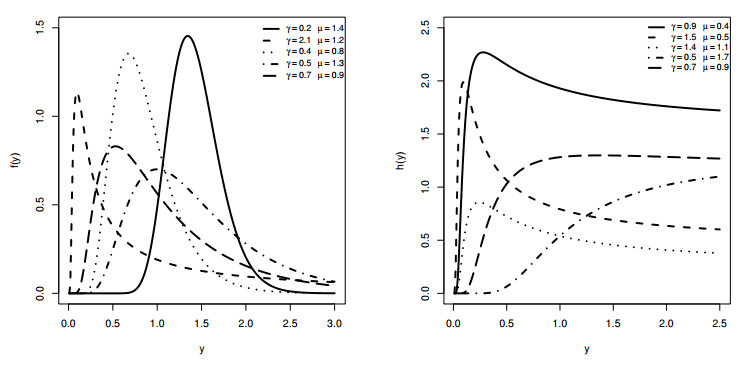
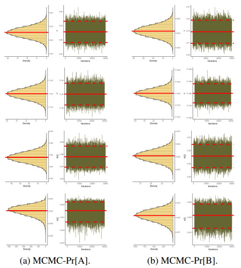
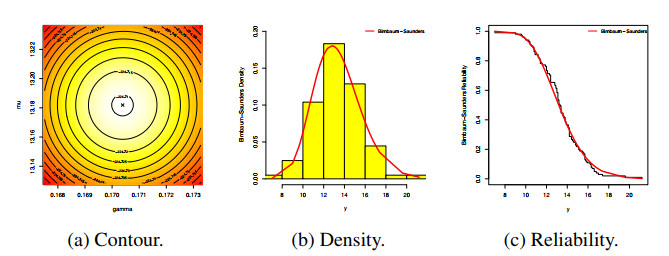
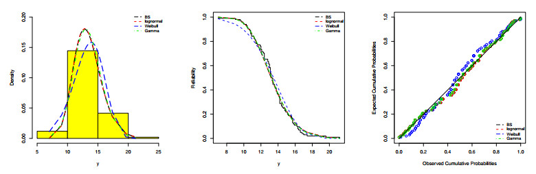
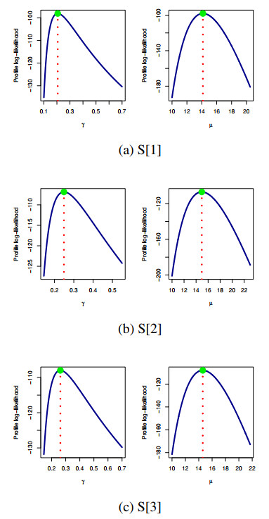
Lately, the Birnbaum-Saunders distribution has gained a lot of attention, mainly due to its different density shapes and the non-monotonicity property of its failure rates. This work considered some estimation issues for the Birnbaum-Saunders distribution using adaptive progressive Type-Ⅱ hybrid censoring. Point and interval estimations were performed employing both conventional and Bayesian methodologies. In addition to estimating the model parameters, we obtained point and interval estimates for the reliability and hazard rate functions. We looked at the method of maximum likelihood as a classical approach, and its asymptotic traits were employed to obtain approximate confidence ranges. From a Bayesian point of perspective, we considered the squared error loss function to obtain the point estimates of the various parameters. The Bayes and highest posterior density credible intervals were additionally determined. For the complex form of the posterior distribution, Bayes estimates and credible intervals were computed by sampling from the posterior distribution through the Markov chain Monte Carlo procedure. For assessing the performance of all of these estimators, a Monte Carlo simulation was employed. Several statistical standards were applied to check the effectiveness of various estimates for multiple levels of censoring with small, moderate, and large sample sizes. Finally, two scenarios for applications were given in order to highlight the usefulness of the supplied approaches.
Citation: Ahmed Elshahhat, Refah Alotaibi, Mazen Nassar. Statistical inference of the Birnbaum-Saunders model using adaptive progressively hybrid censored data and its applications[J]. AIMS Mathematics, 2024, 9(5): 11092-11121. doi: 10.3934/math.2024544
Lately, the Birnbaum-Saunders distribution has gained a lot of attention, mainly due to its different density shapes and the non-monotonicity property of its failure rates. This work considered some estimation issues for the Birnbaum-Saunders distribution using adaptive progressive Type-Ⅱ hybrid censoring. Point and interval estimations were performed employing both conventional and Bayesian methodologies. In addition to estimating the model parameters, we obtained point and interval estimates for the reliability and hazard rate functions. We looked at the method of maximum likelihood as a classical approach, and its asymptotic traits were employed to obtain approximate confidence ranges. From a Bayesian point of perspective, we considered the squared error loss function to obtain the point estimates of the various parameters. The Bayes and highest posterior density credible intervals were additionally determined. For the complex form of the posterior distribution, Bayes estimates and credible intervals were computed by sampling from the posterior distribution through the Markov chain Monte Carlo procedure. For assessing the performance of all of these estimators, a Monte Carlo simulation was employed. Several statistical standards were applied to check the effectiveness of various estimates for multiple levels of censoring with small, moderate, and large sample sizes. Finally, two scenarios for applications were given in order to highlight the usefulness of the supplied approaches.

| [1] |
Z. W. Birnbaum, S. C. Saunders, A probabilistic interpretation of Miner's rule, SIAM J. Appl. Math., 16 (1968), 637–652. https://doi.org/10.1137/0116052 doi: 10.1137/0116052

|
| [2] |
H. K. T. Ng, D. Kundu, N. Balakrishnan, Point and interval estimation for the two-parameter Birnbaum-Saunders distribution based on Type-Ⅱ censored samples, Comput. Stat. Data An., 50 (2006), 3222–3242. https://doi.org/10.1016/j.csda.2005.06.002 doi: 10.1016/j.csda.2005.06.002
|
| [3] |
A. J. Lemonte, F. Cribari-Neto, K. L. P. Vasconcellos, Improved statistical inference for the two-parameter Birnbaum-Saunders distribution, Comput. Stat. Data An., 51 (2007), 4656–4681. https://doi.org/10.1016/j.csda.2006.08.016 doi: 10.1016/j.csda.2006.08.016
|
| [4] |
B. Pradhan, D. Kundu, Inference and optimal censoring schemes for progressively censored Birnbaum-Saunders distribution, J. Stat. Plan. Infer., 143 (2013), 1098–1108. https://doi.org/10.1016/j.jspi.2012.11.007 doi: 10.1016/j.jspi.2012.11.007
|
| [5] |
X. Y. Peng, Y. Xiao, Z. Z. Yan, Reliability analysis of Birnbaum-Saunders model based on progressive type-Ⅱ censoring, J. Stat. Comput. Sim., 89 (2019), 461–477. https://doi.org/10.1080/00949655.2018.1555251 doi: 10.1080/00949655.2018.1555251
|
| [6] |
N. Balakrishnan, D. Kundu, Birnbaum-Saunders distribution: A review of models, analysis, and applications, Appl. Stoch. Model. Bus., 35 (2019), 4–49. https://doi.org/10.1002/asmb.2348 doi: 10.1002/asmb.2348
|
| [7] |
D. Kundu, N. Kannan, N. Balakrishnan, On the hazard function of Birnbaum-Saunders distribution and associated inference, Comput. Stat. Data An., 52 (2008), 2692–2702. https://doi.org/10.1016/j.csda.2007.09.021 doi: 10.1016/j.csda.2007.09.021
|
| [8] | N. Balakrishnan, R. Aggarwala, Progressive censoring: theory, methods, and application, Boston: Birkhäuser, 2000. https://doi.org/10.1007/978-1-4612-1334-5 |
| [9] |
D. Kundu, A. Joarder, Analysis of Type-Ⅱ progressively hybrid censored data, Comput. Stat. Data An., 50 (2006), 2509–2528. https://doi.org/10.1016/j.csda.2005.05.002 doi: 10.1016/j.csda.2005.05.002
|
| [10] |
H. K. T. Ng, D. Kundu, P. S. Chan, Statistical analysis of exponential lifetimes under an adaptive Type‐Ⅱ progressive censoring scheme, Nav. Res. Log., 56 (2009), 687–698. https://doi.org/10.1002/nav.20371 doi: 10.1002/nav.20371
|
| [11] |
M. Nassar, O. E. Abo-Kasem, Estimation of the inverse Weibull parameters under adaptive type-Ⅱ progressive hybrid censoring scheme, J. Comput. Appl. Math., 315 (2017), 228–239. https://doi.org/10.1016/j.cam.2016.11.012 doi: 10.1016/j.cam.2016.11.012
|
| [12] |
R. Alotaibi, A. Elshahhat, H. Rezk, M. Nassar, Inferences for Alpha power exponential distribution using adaptive progressively type-Ⅱ hybrid censored data with applications, Symmetry, 14 (2022), 651. https://doi.org/10.3390/sym14040651 doi: 10.3390/sym14040651
|
| [13] |
H. H. Ahmad, M. M. Salah, M. S. Eliwa, Z. A. Alhussain, E. M. Almetwally, E. A. Ahmed, Bayesian and non-Bayesian inference under adaptive type-Ⅱ progressive censored sample with exponentiated power Lindley distribution, J. Appl. Stat., 49 (2022), 2981–3001. https://doi.org/10.1080/02664763.2021.1931819 doi: 10.1080/02664763.2021.1931819
|
| [14] |
S. Dutta, S. Dey, S. Kayal, Bayesian survival analysis of logistic exponential distribution for adaptive progressive Type-Ⅱ censored data, Comput. Stat., 2023 (2023), 1–47. https://doi.org/10.1007/s00180-023-01376-y doi: 10.1007/s00180-023-01376-y
|
| [15] |
A. Elshahhat, M. Nassar, Analysis of adaptive Type-Ⅱ progressively hybrid censoring with binomial removals, J. Stat. Comput. Sim., 93 (2023), 1077–1103. https://doi.org/10.1080/00949655.2022.2127149 doi: 10.1080/00949655.2022.2127149
|
| [16] |
J. A. Achcar, Inferences for the Birnbaum-Saunders fatigue life model using Bayesian methods, Comput. Stat. Data An., 15 (1993), 367–380. https://doi.org/10.1016/0167-9473(93)90170-X doi: 10.1016/0167-9473(93)90170-X
|
| [17] |
A. C. Xu, Y. C. Tang, Reference analysis for Birnbaum-Saunders distribution, Comput. Stat. Data An., 54 (2010), 185–192. https://doi.org/10.1016/j.csda.2009.08.004 doi: 10.1016/j.csda.2009.08.004
|
| [18] |
J. E. Contreras-Reyes, F. O. L. Quintero, R. Wiff, Bayesian modeling of individual growth variability using back-calculation: Application to pink cusk-eel (Genypterus blacodes) off Chile, Ecol. Model., 385 (2018), 145–153. https://doi.org/10.1016/j.ecolmodel.2018.07.002 doi: 10.1016/j.ecolmodel.2018.07.002
|
| [19] |
A. Henningsen, O. Toomet, maxLik: A package for maximum likelihood estimation in R, Comput. Stat., 26 (2011), 443–458. https://doi.org/10.1007/s00180-010-0217-1 doi: 10.1007/s00180-010-0217-1
|
| [20] | M. Plummer, N. Best, K. Cowles, K. Vines, Coda: Convergence diagnosis and output analysis for MCMC, R. News, 6 (2006), 7–11. |
| [21] |
D. M. Hawkins, Diagnostics for conformity of paired quantitative measurements, Stat. Med., 21 (2002), 1913–1935. https://doi.org/10.1002/sim.1013 doi: 10.1002/sim.1013
|
| [22] |
M. Nassar, R. Alotaibi, A. Elshahhat, Complexity analysis of E-Bayesian estimation under type-Ⅱ censoring with application to organ transplant blood data, Symmetry, 14 (2022), 1308. https://doi.org/10.3390/sym14071308 doi: 10.3390/sym14071308
|
| [23] |
H. K. T. Ng, D. Kundu, N. Balakrishnan, Modified moment estimation for the two-parameter Birnbaum-Saunders distribution, Comput. Stat. Data An., 43 (2003), 283–298. https://doi.org/10.1016/S0167-9473(02)00254-2 doi: 10.1016/S0167-9473(02)00254-2
|
Figures(9) / Tables(18)

Ahmed Elshahhat, Refah Alotaibi, Mazen Nassar. Statistical inference of the Birnbaum-Saunders model using adaptive progressively hybrid censored data and its applications[J]. AIMS Mathematics, 2024, 9(5): 11092-11121. doi: 10.3934/math.2024544


 DownLoad: