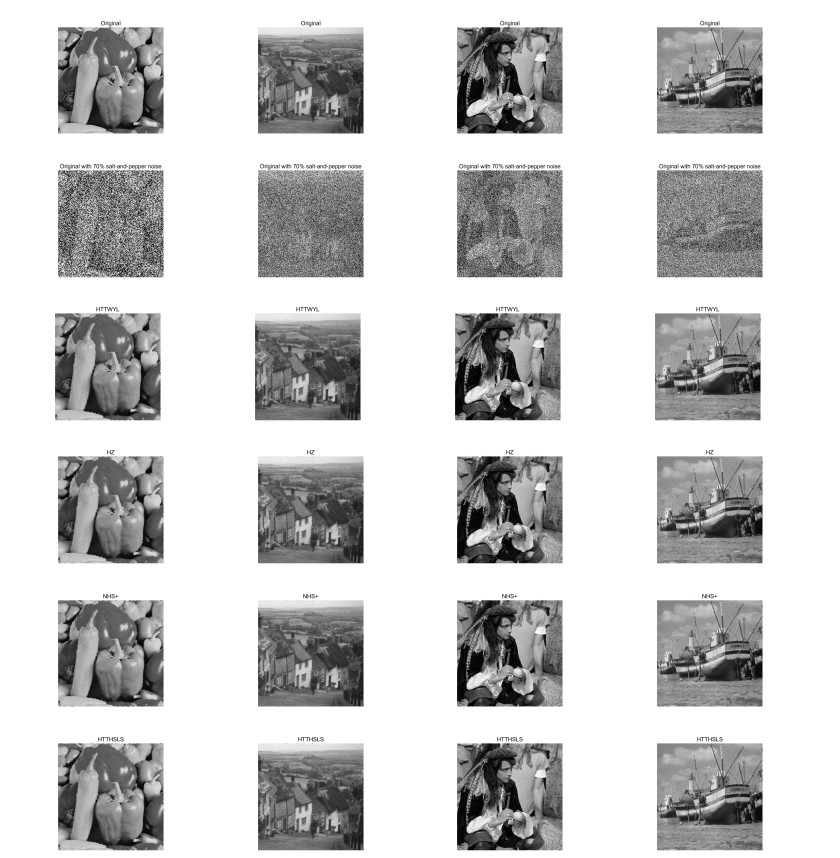
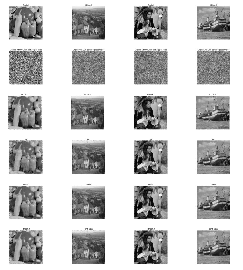
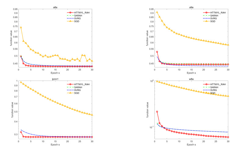
A new hybrid conjugate gradient method close to the memoryless BFGS quasi-Newton method and its application in image restoration and machine learning

1.   Introduction

In this work, we consider the following unconstrained optimization problem:

where $f:\mathbb R^n \to \mathbb R$ is continuously differentiable and bounded below. Conjugate gradient methods are highly significant for solving large-scale optimization due to their lower storage requirements and simple computation. They are widely applied in various fields, including information technology ^[1], energy engineering ^[2,3], material science ^[4,5], and more. The conjugate gradient method for solving (1.1) generates an iterate sequence $\{x_k\}$ using the formula

where the scalar $\alpha_k > 0$ is the step size and satisfies the Wolfe line search conditions

where $g_{k} = \bigtriangledown f(x_{k})$, $0 < \rho \le \sigma \le 1$. The search direction $d_k$ is generally given by

where $\beta_k \in \mathbb{R}^{n}$ is the conjugate parameter.

Some of the famous conjugate gradient methods are the Fletcher-Reeves (FR) method ^[6], the Polak-Ribiere-Polyak (PRP) method ^[7,8], the Hestenes-Stiefel (HS) method ^[9], and the Dai-Yuan (DY) method ^[10], the Liu–Storey (LS) method ^[11], and their parameters $\beta_{k}$ are, respectively,

where $y_{k-1} = g_{k}-g_{k-1}$. $\left \| \cdot \right \|$ represents the Euclidean norm.

Different conjugate parameter choices lead to variants of the conjugate gradient method, each with its own unique strengths and differences in theoretical convergence and numerical performance. In recent years, the modified conjugate gradient method ^{[12,13,14,15]} and hybrid conjugate gradient method ^[16,17] have received much attention. Their researches exhibited better convergence properties and broader applications and illustrated the significance of our in-depth study of the conjugate gradient method.

In 2006, Wei et al. ^[18] proposed a modification of the PRP conjugate gradient method, denoted as the Wei-Yao-Liu (WYL) method by substituting $y_{k-1}$ with $y_{k-1}^* = g_k-\frac{\|g_k\|}{\|g_{k-1}\|}g_{k-1}$ in $\beta_k^{PRP}$, and introduced the new conjugate parameter

When the normalized gradient difference $y_{k-1}^*$ tended to zero, leading that the scalar $\beta_k^{WYL}$ also approached to zero, which in turn caused the search direction to be close to the steepest descent direction{, it} implied that the WYL method possessed the automatic restart feature, similar to the PRP method. Furthermore, when the gradients $g_k$ and $g_{k-1}$ were significantly different, the smaller one between $g_{k}$ and $g_{k-1}$ was almost negligible in the computation of $y_{k-1}$. The fact $\|\frac{\|g_k\|}{\|g_{k-1}\|}g_{k-1}\| = \|g_k\|$ guaranteed that the vector $y_{k-1}^*$ could utilize the available information both of $g_{k}$ and $g_{k-1}$ and enhanced the numerical stability. More researches on $y_{k-1}^*$ could be found in ^{[12,13,14,16,19]}.

In recent years, the memoryless BFGS method has been commonly employed in constructing the hybrid conjugate gradient method. In 2018, Li ^[15] rewrote the memeoryless BFGS update $d_k^{BFGS}$ in ^[20] as

and proposed a new conjugate direction by closing to the memoryless BFGS quasi-Newton method

where $t_k$ was established by minimizing the distance between $(y_{k-1}-s_{k-1})$ and $t_ky_{k-1}$. Moreover, such a constructed conjugate gradient method was considered as a three-term conjugate gradient method determined by vectors $g_k, d_{k-1}$, and $y_{k-1}$. The method retains the advantages of the HS method and memoryless BFGS method, and it was also suitable for large-scale optimization problems.

In 2023, Kumam ^[17] presented a hybrid conjugate gradient method for solving (1.1). The direction combines the three-term PRP, HS, and LS directions.

where

and $t_k$ is as well as that of (1.7). Furthermore, the direction was close to the memoryless BFGS quasi-Newton method and had the descent and trust region properties.

In addition, conjugate gradient methods have been employed to deal with the image restoration efficiently. In 2020, Luo et. al ^[21] proposed a conjugate gradient algorithm based on double parameter scaled BFGS and applied it to solve image restoration problems. In 2023, Jiang et. al ^[22] proposed a family of hybrid conjugate gradient methods with restart procedure for unconstrained optimizations and image restorations. In 2024, Jiang et. al ^[23] put forward a family of spectral conjugate gradient methods with strong convergence and its applications in image restoration and machine learning. More related researches are detailed in the references ^{[21,24,25,26,27]}.

Inspired by the above works, we present a hybrid conjugate gradient method by constructing new combined conjugate parameters for solving (1.1). The main contributions of this paper are stated as follows.

$\bullet$ The new method can be viewed as a three-term conjugate gradient method in which the search direction is a linear combination of $g_k, d_{k-1}, y_{k-1}^*$. Their coefficients are defined as a combination of PRP, HS, LS, {and} WYL conjugate paremeters. The new direction is close to the memoryless BFGS quasi-Newton direction.

$\bullet$ The search directions generated by the proposed method satisfy the sufficient descent condition independent of any line search. Under usual assumptions and the Wolfe line search, the global convergence of our algorithm is proved.

$\bullet$ Numerical experiments of the proposed method are carried out for solving unconstrained test problems, and we apply the new method in the image restoration problems and machine learning problems.

The rest of this paper is organized as follows. In the next section, we put forward a new hybrid three-term conjugate gradient method and provide a framework of the algorithm. The sufficient descent property and global convergence are demonstrated in Section 2. In Section 3, some numerical experiments are implemented for solving some unconstrained test problems. In Section 4, we use the new algorithm to solve image restoration problems. In Section 5, a conclusion for this work is made.

2.   New algorithm and convergence analysis

In this work, motivated by the three-term conjugate gradient direction defined in (1.8) and taking the advantage of the $\beta_k^{WYL}$ and $y_{k-1}^*$ in ^[18], we define a new three-term hybrid conjugate gradient method with the following search direction:

where

and

When $\eta_k = \|g_{k-1}\|^2$, $\beta_k = \beta_k^{WYL}-\frac{\|y_{k-1}^*\|^2g_k^Td_{k-1}}{\eta_k^2}$ could be regarded as a modification of $\beta_k^{WYL}$.

To obtain the parameter $t_k$, similar to the treatment of $t_k$ in (1.7), we require the solution of the univariate minimal problem

Setting $M_k = (y_{k-1}-s_{k-1})-t\cdot y_{k-1}^*$,

Setting $A_k = y_{k-1}-s_{k-1}$,

and

Taking the derivative of the above equation and setting it equal to zero, we obtain

which implies

Therefore, we choose $t_k$ as

which implies $0\leq t_k\leq\bar{t} < 1$. Note that the direction defined by (2.1) is close to the direction of the memoryless BFGS method when $t_k$ is chosen by (2.3).

Based on the above analysis, the new algorithm can be presented as follows.

Algorithm 1 (HTTWYL)

Step 0: Input $x_0\in \mathbb{R} ^n$, parameters $\varepsilon > 0$, $0 < \rho < \sigma < 1$. $d_{1} = -g_{1}$, set $k: = 1$;

Step 1: If $\|g_k\|\le \varepsilon$, then stop.

Step 2: Determine a step-length $\alpha_k$ by the Wolfe line search (1.2) and (1.3);

Step 3: Let $x_{k+1} = x_k+\alpha_kd_k$, calculate $g_{k+1}$, $f(x_{k+1})$;

Step 4: Determine $t_k$, $\gamma_k$, and $\beta_k$ as in (2.4) and (2.2), respectively. Compute the search direction as in (2.1).

Step 5: Set $k: = k+1$, and go to Step 1.

The following lemma shows that the $d_k$ produced by (2.1) satisfies the property of sufficient descent without any line search.

Lemma 2.1. If $\{d_k\}$ is defined by (2.1), then we obtain

where $c_1 = \left(1-\frac{(1+\bar{t})^2}4\right)$.

Proof.

so the proof is complete. ■

Next, we will attempt to establish the convergence of the standard Wolfe line search conditions. We use the following assumptions.

Assumption 1. The level set $D = \left \{ x\in \mathbb R^n:f\left (x \right) \le f \left (x_0 \right) \right \}$ is bounded. It means

Assumption 2. The gradient function $g\left (x \right)$ is Lipschitz continuous on the level set $D$, exists a constant $L$, s.t.,

Based on the above assumptions, it can be {shown} that there exists a constant $\Gamma > 0$ such that

Theorem 2.1. Let the sequence $\{x_k\}$ be generated by Algorithm 1, and suppose the Assumptions 1 and 2 holds, If

then

Proof. By paradoxically assuming that (2.7) does not hold, then there exists a nonnegative constant $\zeta$ such that

From (2.2), we have

Also,

Then, from formula (2.1), (2.9), and (2.10), we obtain

Letting $M_1 = \left(1+\frac{1+\bar{t}}\mu+\frac1{\mu^2}\right)\Gamma$, we have

From Lemma 2.1, the first Wolfe condition (1.2), and (2.8),

Conjugating with Assumption 1, the sequence $\{f(x_k)\}$ is convergent.

From the second Wolfe condition (1.3) and Assumption 2, we obtain

Using the above inequality and (1.2), we derive

Summing both sides of the above equation for $k = 0, 1, ..., K$, we get

Let $K\to \infty$, and the above implies that

Now, combining (2.8) with (2.5), we get

Therefore, we have

this contradicts (2.6). Then, (2.7) holds. ■

3.   Numerical experiments

In this section, we compare the computational performance of HTTWYL with the method proposed by Hager and Zhang ^[28] (HZ), the method proposed by MinLi ^[15] (NHS+), and the method by Kumam ^[17] (HTTHSLS) under standard Wolfe line search. All codes are written on Matlab R2022a and run on a PC with the 2200MHz central processing unit (CPU) processor, 16.00 GB RAM memory.

Most of the test functions were drawn from the Constrained and Unconstrained Testing Environment, revisited (CUTEr) library ^[29], and some test functions were suggested by Andrei ^[30] and Moré et al. ^[31]. Table 1 lists 49 test functions for 100 problems with dimensions from 10 to 1000000. The parameters for the four methods are selected in the following manner.

All algorithms are terminated when it satisfies the condition $\|g_k\|\le \epsilon$ or the number of iterations exceeds 2000. Table 2 lists the numerical results of the four algorithms for 100 test problems. If the Itr exceeds 2000 and the method never reaches the optimal value, the algorithm stops and we write it as "F". The detailed numerical results are listed in the form Itr, Nf, $\|g_*\|$, and Tcpu, where it denotes the number of iterations, function evaluations, the gradient value at the end of iteration, and the CPU time, respectively.

We use the performance profile introduced by Dolan and More ^[32] to analyze the computational performance of all methods. Let $P$ be the collection of $n_p$ test problems and $S$ be the set of solvers used in the comparison. The measure $t_{p, s}$ is defined as Itr, Nf, or Tcpu required by solver $s$ for problem $p$. The definition of the performance ratio is

It is obvious that $r_{p, s} \ge 1$ for all $p$ and $s$. The performance profiles for each solver $s$ {are} defined by

where $size\{p\in P:r_{p, s}\leq\tau\}$ is the number of the elements in the set $\{p\in P:r_{p, s}\leq\tau\}$, then $P(\tau)$ is the probability for solver $s \in S$ that a performance ratio $r_{p, s}$ is within a factor $\tau$. The efficiency of a method is represented on the horizontal axis by the percentage $\tau$ of test problems for which it is the fastest, while the vertical axis indicates the success rate $P(\tau)$ of each method in solving the test problems.

Figure 1 illustrates the iteration performance profiles of the methods. It demonstrates that most of the positions of the curves of our proposed algorithm lie above the curves of the other three methods, and our algorithm can successfully solve about 99% of the test problems. The HZ method solves about 90%, the NHS+ method solves about 87%, and the HTTHSLS method solves about 87% of the test problems, respectively. Figure 2 shows the curve of the HTTWYL method is above those of the other methods. This indicates the HTTWYL method wins the match in the function evaluations. Similarly, Figure 3 shows the HTTWYL method wins the performance profiles on CPU time, and we can see that the HTTWYL method outperforms the other three methods for the given test set. In brief, by observing the overall trend in the performance graphs, the HTTWYL algorithm performs slightly better than other algorithms. We believe that the HTTWYL algorithm is more competitive.

4.   Application in image restoration

In this section, we use the HTTWYL algorithm to solve image restoration problems. Cai et al.^[33] used the two-phase scheme to clean salt-and-pepper noise. The first phase is to detect noisy pixels by using the adaptive median filter ^[34]. The second phase involves clearing noisy pixels by solving the following smoothing minimization problem.

Here, $\varphi_\chi(t) = \sqrt{t^2+\chi}$ is an edge-preserving function with parameter $\alpha > 0$. $\mathcal{N}\subset\mathcal{A}$ is the index set of noise pixels detected in the first phase, $\mathcal{A} = \{1, \ldots, M\}\times\{1, \ldots, N\}$ is the pixel pointer set of the original image of size $M\times N$, $\mathbf{u} = [u_{i, j}]_{(i, j)\in\mathcal{N}}$ is a column vector of length $|\mathcal{N}|$ ordered lexicographically, i.e., the number of elements in ${\mathcal{N}}$, and $y_{i, j}$ is the pixel value of the image at the point $(i, j)$.

Now, our attention shifts to employing the two-phase strategy to eliminate salt-and-pepper noise, which is a specific instance of impulse noise. In the first phase, we employ an adaptive median filter ^[34] to identify noisy pixels. Obviously, the higher the noise ratio, the larger the scale of (4.1). Cai ^[33] discovered that the contaminated images can be restored efficiently by using the conjugate gradient methods to solve the above problem (4.1). Thus, in the second phase, we utilize the HTTWYL method to solve (4.1) and continue to compare it with the HZ, NHS+, and HTTHSLS methods. These methods all use the Wolfe line search (1.2) and (1.3) to compute the step-length $\alpha_k$. Moreover, the related parameters for these methods are set as follows: $\rho = 0.1, \ \sigma = 0.01,$ $\bar t = 0.3.$

The test images are Peppers(512 × 512), Hill(512 × 512), Man(512 × 512), and Boat(512 × 512). The stopping criterion for the involved methods is

In order to evaluate the restoration performance clearly, we use the peak signal to noise ratio (PSNR; see ^[35]) defined by

where $x_{i, j}^r$ and $x_{i, j}^*$ represent the pixel values of the restored image and the original one, respectively.

We plot the original, noisy, and restored images for three algorithms when the salt-and-pepper noise ratio is 70% and 90%. For the corresponding results, see Figures 4 and 5. In Table 3, we report the number of iterations (Itr), the CPU time (Tcpu), and the PSNR values. From Table 3, we can intuitively perceive that the HTTWYL method usually has higher PSNR among the three methods under the same noise ratio, and it takes fewer iterations and CPU time than the other three methods in most cases. Thus, our algorithm seems to be capable to reconstruct the noisy pictures with more quality.

5.   Application in machine learning problem

In this section, we test the numerical performance of the HTTWYL in solving the machine learning problem. We embed the HTTWYL algorithm into the stochastic recursive gradient algorithm (SARAH) ^[36] (denote as HTTWYL_RAH). We use the Wolfe line search criterion to calculate the learning rate (step size). In addition, we compare the HTTWYL_RAH method with the stochastic variance reduced gradient (SVRG) ^[37], SARAH, and stochastic gradient descent (SGD) ^[38] methods. All the experiments tested the following learning model:

Ridge regression (ridge)

where $y_i\in\{-1, +1\}$ is the target value of the $i$th sample and $x_i \in R^d$ is a feature vector of the $i$th sample. $\lambda > 0$ is a regularization parameter. The related parameters for these methods are set as follows: $\rho = 0.1, \ \sigma = 0.01, \bar t = 0.3.$ All algorithms are executed on four large-scale datasets, including a8a, a9a, ijcnn1, and w8a. These datasets come from the LIBSVM Data website ^*, and the specific details of the datasets are provided in Table 4. The vertical axis represents the function value of the loss value and the horizontal axis represents the number of internal iterations. The parameters in SARAH, SVRG, SGD are the same as their original papers. In this experiment, the maximum number of inner iterations is 30. Figure 6 represents the convergence of the loss function ($\lambda$ = $10^{-2}$) for six algorithms on four datasets.

^*All datasets are available at https://www.csie.ntu.edu.tw/cjlin/libsvmtools/datasets/.

In general, a lower curve of the algorithm indicates better convergence behavior. As can be seen in Figure 6, the HTTWYL_RAH method has the fastest convergence in most cases.

6.   Conclusions

We present a hybrid three-term conjugate gradient method HTTWYL for solving unconstrained optimization problems, which combines features from WYL and other classical conjugate gradient methods. The global convergence of the method is established under certain conditions. We use it to deal with the unconstrained optimization test problems and apply it to solving image restoration problems and ridge regression in machine learning problems. The numerical results indicate that compared to other methods, our proposed method is more effective and promising. Finally, we hope that the contributions in this paper will continue to be explored for applications in other areas.

Author contributions

Zhang and Yang: Writing-original draft and editing. All authors have read and approved the final version of the manuscript for publication.

Acknowledgments

This research is funded by the Science and Technology Development Planning Grant Program of Jilin Province (YDZJ202101ZYTS167, 20200403193SF), and the graduate innovation project of Beihua University (2023035, 2022038).

Conflict of interest

All authors declare no conflicts of interest in this paper.