An efficient spectral minimization of the Dai-Yuan method with application to image reconstruction

Nasiru Salihu; Poom Kumam; Ibrahim Mohammed Sulaiman; Thidaporn Seangwattana; Nasiru Salihu; Poom Kumam; Ibrahim Mohammed Sulaiman; Thidaporn Seangwattana

doi:10.3934/math.20231583

AIMS Mathematics

2023, Volume 8, Issue 12: 30940-30962. doi: 10.3934/math.20231583

Previous Article Next Article

Research article

An efficient spectral minimization of the Dai-Yuan method with application to image reconstruction

1.
Center of Excellence in Theoretical and Computational Science (TaCS-CoE), Fixed Point Research Laboratory, Fixed Point Theory and Applications Research Group, Faculty of Science, King Mongkut's University of Technology Thonburi (KMUTT), Bangkok 10140, Thailand
2.
Department of Mathematics, Faculty of Sciences, Modibbo Adama University, Yola 652105, Nigeria
3.
KMUTT-Fixed Point Research Laboratory, Room SCL 802, Science Laboratory Building, Department of Mathematics, Faculty of Science, King Mongkut's University of Technology Thonburi (KMUTT), Bangkok 10140, Thailand
4.
Institute of Strategic Industrial Decision Modelling, School of Quantitative Sciences, Universiti Utara Malaysia, Sintok, Kedah 06010, Malaysia
5.
Faculty of Education and Arts, Sohar University, Sohar 311, Oman
6.
Faculty of Science Energy and Environment, King Mongkut's University of Technology North Bangkok, Rayong Campus (KMUTNB), Rayong 21120, Thailand

Received: 16 August 2023 Revised: 24 September 2023 Accepted: 13 October 2023 Published: 17 November 2023
MSC : 65K05, 90C06, 90C30, 90C47, 90C90

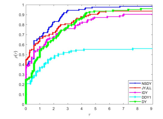
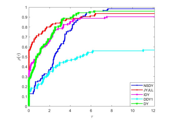
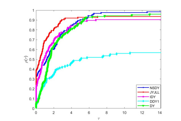
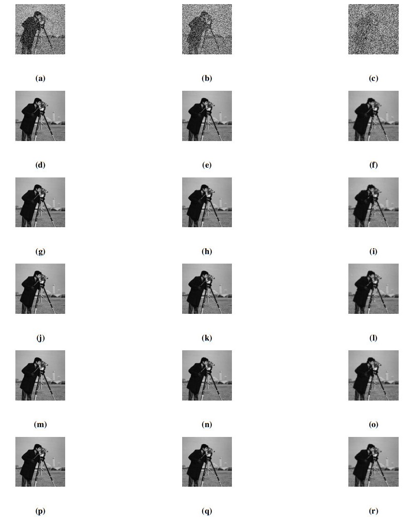
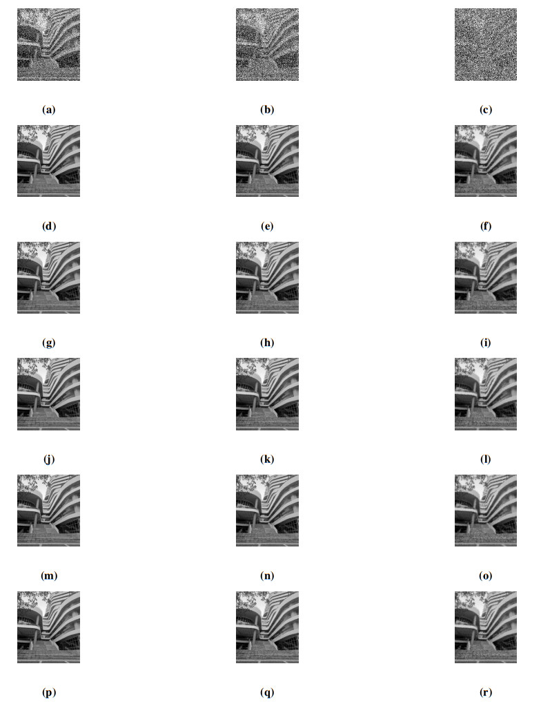
In this paper, a spectral Dai and Yuan conjugate gradient (CG) method is proposed based on the generalized conjugacy condition for large-scale unconstrained optimization, in which the spectral parameter is motivated by some interesting theoretical features of quadratic convergence associated with the Newton method. Accordingly, utilizing the strong Wolfe line search to yield the step-length, the search direction of the proposed spectral method is sufficiently descending and converges globally. By applying some standard Euclidean optimization test functions, numerical results reports show the advantage of the method over some modified Dai and Yuan CG schemes in literature. In addition, the method also shows some reliable results, when applied to solve an image reconstruction model.
- unconstrained optimization,
- spectral conjugate gradient method,
- generalized conjugacy condition,
- Newton direction,
- global convergence,
- image reconstruction
Citation: Nasiru Salihu, Poom Kumam, Ibrahim Mohammed Sulaiman, Thidaporn Seangwattana. An efficient spectral minimization of the Dai-Yuan method with application to image reconstruction[J]. AIMS Mathematics, 2023, 8(12): 30940-30962. doi: 10.3934/math.20231583

Related Papers:

Abstract

In this paper, a spectral Dai and Yuan conjugate gradient (CG) method is proposed based on the generalized conjugacy condition for large-scale unconstrained optimization, in which the spectral parameter is motivated by some interesting theoretical features of quadratic convergence associated with the Newton method. Accordingly, utilizing the strong Wolfe line search to yield the step-length, the search direction of the proposed spectral method is sufficiently descending and converges globally. By applying some standard Euclidean optimization test functions, numerical results reports show the advantage of the method over some modified Dai and Yuan CG schemes in literature. In addition, the method also shows some reliable results, when applied to solve an image reconstruction model.

References

[1]	I. M. Sulaiman, M. Malik, A. M. Awwal, P. Kumam, M. Mamat, S. Al-Ahmad, On three-term conjugate gradient method for optimization problems with applications on covid-19 model and robotic motion control, Adv. Contin. Discrete Models, (2022), 1–22.
[2]	N. Salihu, P. Kumam, A. M. Awwal, I. Arzuka, T. Seangwattana, A Structured Fletcher-Revees Spectral Conjugate Gradient Method for Unconstrained Optimization with Application in Robotic Model, In Operations Research Forum, 4 (2023), 81.
[3]	K. Kamilu, M. Sulaiman, A. Muhammad, A. Mohamad, M. Mamat, Performance evaluation of a novel conjugate gradient method for training feed forward neural network, Math. Model. Comp., 10 (2023), 326–337.
[4]	M. M. Yahaya, P. Kumam, A. M. Awwal, P. Chaipunya, S. Aji, S. Salisu, A new generalized quasi-newton algorithm based on structured diagonal Hessian approximation for solving nonlinear least-squares problems with application to 3dof planar robot arm manipulator, IEEE Access, 10 (2022), 10816–10826. https://doi.org/10.1109/ACCESS.2022.3144875 doi: 10.1109/ACCESS.2022.3144875
[5]	A. S. Halilu, A. Majumder, M. Y. Waziri, K. Ahmed, Signal recovery with convex constrained nonlinear monotone equations through conjugate gradient hybrid approach, Math. Comput. Simul., 187 (2021), 520–539.
[6]	I. M. Sulaiman, M. Mamat, A new conjugate gradient method with descent properties and its application to regression analysis, JNAIAM. J. Numer. Anal. Ind. Appl. Math., 14 (2020), 25–39.
[7]	G. Yuan, J. Lu, Z. Wang, The PRP conjugate gradient algorithm with a modified WWP line search and its application in the image restoration problems, Appl. Numer. Math., 152 (2020), 1–11.
[8]	N. Salihu, P. Kumam, A. M. Awwal, I. M. Sulaiman, T. Seangwattana, The global convergence of spectral RMIL conjugate gradient method for unconstrained optimization with applications to robotic model and image recovery, Plos one, 18 (3), e0281250.
[9]	M. Malik, I. M. Sulaiman, A. B. Abubakar, G. Ardaneswari, Sukono, A new family of hybrid three-term conjugate gradient method for unconstrained optimization with application to image restoration and portfolio selection, AIMS Math., 8 (2023), 1–28.
[10]	N. Andrei, A Dai-Liao conjugate gradient algorithm with clustering of eigenvalues, Numer. Algorithms, 77 (4), 1273–1282.
[11]	W. W. Hager, H. Zhang, A survey of nonlinear conjugate gradient methods, Pac. J. Optim., 2 (2006), 35–58.
[12]	R. Fletcher, C. M. Reeves, Function minimization by conjugate gradients, Comput. J., 7 (1964), 149–154. https://doi.org/10.1093/comjnl/7.2.149 doi: 10.1093/comjnl/7.2.149
[13]	Y. H. Dai, Y. Yuan, A nonlinear conjugate gradient method with a strong global convergence property, SIAM J. Optim., 10 (1999), 177–182. https://doi.org/10.1137/S1052623497318992 doi: 10.1137/S1052623497318992
[14]	R. Fletcher, Practical methods of optimization, A Wiley-Interscience Publication. John Wiley & Sons, Ltd., Chichester, second edition, 1987.
[15]	X. Du, P. Zhang, W. Ma, Some modified conjugate gradient methods for unconstrained optimization, J. Comput. Appl. Math., 305 (2016), 92–114.
[16]	M. J. D. Powell, Restart procedures for the conjugate gradient method, Math. Program., 12 (1997), 241–254. https://doi.org/10.1023/A:1007963324520 doi: 10.1023/A:1007963324520
[17]	G. Zoutendijk, Nonlinear programming, computational methods, In: J. Abadie Ed., Integer and Nonlinear Programming, North-Holland, Amsterdam, 37–86, 1970.
[18]	N. Andrei, An adaptive scaled BFGS method for unconstrained optimization, Numer. Algorithms, 77 (2018), 413–432. https://doi.org/10.1007/s11075-017-0321-1 doi: 10.1007/s11075-017-0321-1
[19]	Y. H. Dai, L. Z. Liao, New conjugacy conditions and related nonlinear conjugate gradient methods, Appl. Math. Optim., 43 (2001), 87–101.
[20]	M. Raydan, The Barzilai and Borwein gradient method for the large scale unconstrained minimization problem, SIAM J. Optim., 7 (1997), 26–33. https://doi.org/10.1137/S1052623494266365 doi: 10.1137/S1052623494266365
[21]	J. Barzilai, J. M. Borwein, Two-point step size gradient methods. IMA J. Numer. Anal., 8 (1988), 141–148. https://doi.org/10.1093/imanum/8.1.141
[22]	E. G. Birgin, J. M. Martínez, A spectral conjugate gradient method for unconstrained optimization, Appl. Math. Optim., 43 (2001), 117–128.
[23]	N. Salihu, M. R. Odekunle, A. M. Saleh, S. Salihu. A Dai-Liao hybrid Hestenes-Stiefel and Fletcher-Revees methods for unconstrained optimization, Int. J. Indu. Optim., 2 (2021), 33–50.
[24]	N. Salihu, M. Odekunle, M. Waziri, A. Halilu, A new hybrid conjugate gradient method based on secant equation for solving large scale unconstrained optimization problems, Iran. J. Optim., 12 (2020), 33–44. https://doi.org/10.11606/issn.1984-5057.v12i2p33-44 doi: 10.11606/issn.1984-5057.v12i2p33-44
[25]	S. Nasiru, R. O. Mathew, Y. W. Mohammed, S. H. Abubakar, S. Suraj, A Dai-Liao hybrid conjugate gradient method for unconstrained optimization, Int. J. Indu. Optim., 2 (2021), 69–84.
[26]	T. Barz, S. Körkel, G. Wozny, Nonlinear ill-posed problem analysis in model-based parameter estimation and experimental design, Compu. Chem. Engi., 77 (2015), 24–42.
[27]	A. M. Awwal, I. M. Sulaiman, M. Maulana, M. Mustafa, K. Poom, S. Kanokwan, A spectral RMIL+ conjugate gradient method for unconstrained optimization with applications in portfolio selection and motion control, IEEE Access, 9 (2021), 75398–75414. https://doi.org/10.1109/ACCESS.2021.3081570 doi: 10.1109/ACCESS.2021.3081570
[28]	H. Shao, H. Guo, X. Wu, P. Liu, Two families of self-adjusting spectral hybrid DL conjugate gradient methods and applications in image denoising, Appl. Math. Model., 118 (2023), 393–411.
[29]	J. Jian, P. Liu, X. Jiang, C. Zhang, Two classes of spectral conjugate gradient methods for unconstrained optimizations, J. Appl. Math. Comput., 68 (2022), 4435–4456. https://doi.org/10.1007/s12190-022-01713-2 doi: 10.1007/s12190-022-01713-2
[30]	J. Jian, P. Liu, X. Jiang, B. He, Two improved nonlinear conjugate gradient methods with the strong Wolfe line search, Bull. Iranian Math. Soc., 48 (2022), 2297–2319. https://doi.org/10.1007/s41980-021-00647-y doi: 10.1007/s41980-021-00647-y
[31]	I. Arzuka, M. R. Abu Bakar, W. J. Leong, A scaled three-term conjugate gradient method for unconstrained optimization, J. Ineq. Appl., (2016), 1–16. https://doi.org/10.15600/2238-1244/sr.v16n42p1-10
[32]	X. Jiang, J. Jian, Improved Fletcher-Reeves and Dai-Yuan conjugate gradient methods with the strong Wolfe line search, J. Comput. Appl. Math., 34 (2019), 525–534.
[33]	J. Jian, L. Yang, X. Jiang, P. Liu, M. Liu, A spectral conjugate gradient method with descent property, Mathematics, 8 (2020), 280.
[34]	J. Jian, L. Han, X. Jiang, A hybrid conjugate gradient method with descent property for unconstrained optimization, Appl. Math. Model., 39 (2015), 1281–1290. https://doi.org/10.1016/j.apm.2014.08.008 doi: 10.1016/j.apm.2014.08.008
[35]	X. Zhou, L. Lu, The global convergence of modified DY conjugate gradient methods under the wolfe line search, J. Chongqing Normal Univ.(Nat. Sci. Ed.), 33 (2016), 6–10.
[36]	Z. Zhu, D. Zhang, S. Wang, Two modified DY conjugate gradient methods for unconstrained optimization problems, Appl. Math. Comput., 373 (2020), 125004. https://doi.org/10.1016/j.amc.2019.125004 doi: 10.1016/j.amc.2019.125004
[37]	N. Andrei, Nonlinear conjugate gradient methods for unconstrained optimization, volume 158 of Springer Optimization and Its Applications, Springer, Cham, 2020.
[38]	J. Momin, Y. X. She, A literature survey of benchmark functions for global optimization problems, Int. J. Mathe. Model. Nume. Optim., 4 (2013), 150–194.
[39]	E. D. Dolan, J. J. Moré, Benchmarking optimization software with performance profiles, Math. Program., 91 (2002), 201–213. https://doi.org/10.1007/s101070100263 doi: 10.1007/s101070100263
[40]	M. Nadipally, Chapter 2-Optimization of methods for image-texture segmentation using ant colony optimization, volume 1, In: Intelligent Data Analysis for Biomedical Applications, Academic Press, Elsevier, 2019.
[41]	G. Yu, J. Huang, Y. Zhou, A descent spectral conjugate gradient method for impulse noise removal, Appl. Math. Lett., 23 (2010), 555–560. https://doi.org/10.1016/S0268-005X(08)00209-9 doi: 10.1016/S0268-005X(08)00209-9

Reader Comments

Your name:*

Email:*
© 2023 the Author(s), licensee AIMS Press. This is an open access article distributed under the terms of the Creative Commons Attribution License (http://creativecommons.org/licenses/by/4.0)