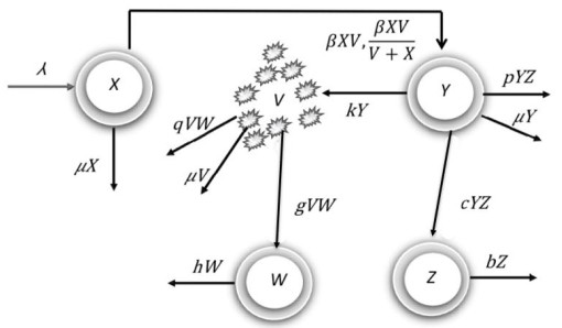
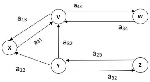
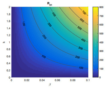
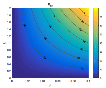
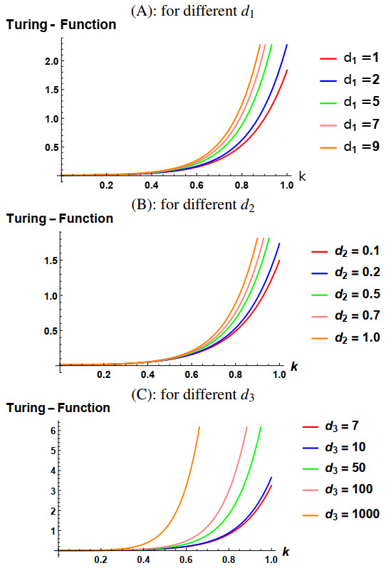
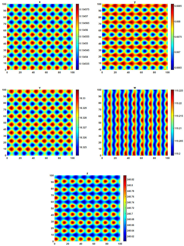
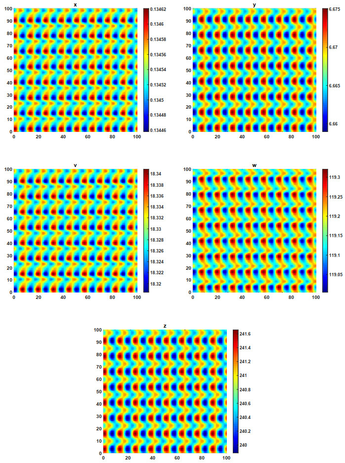
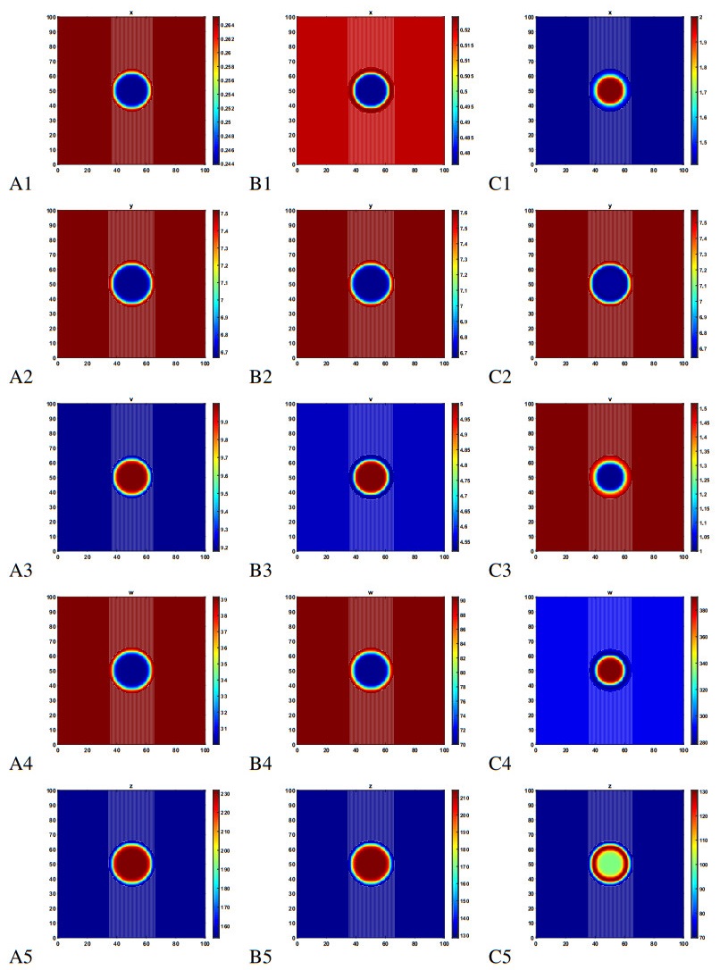
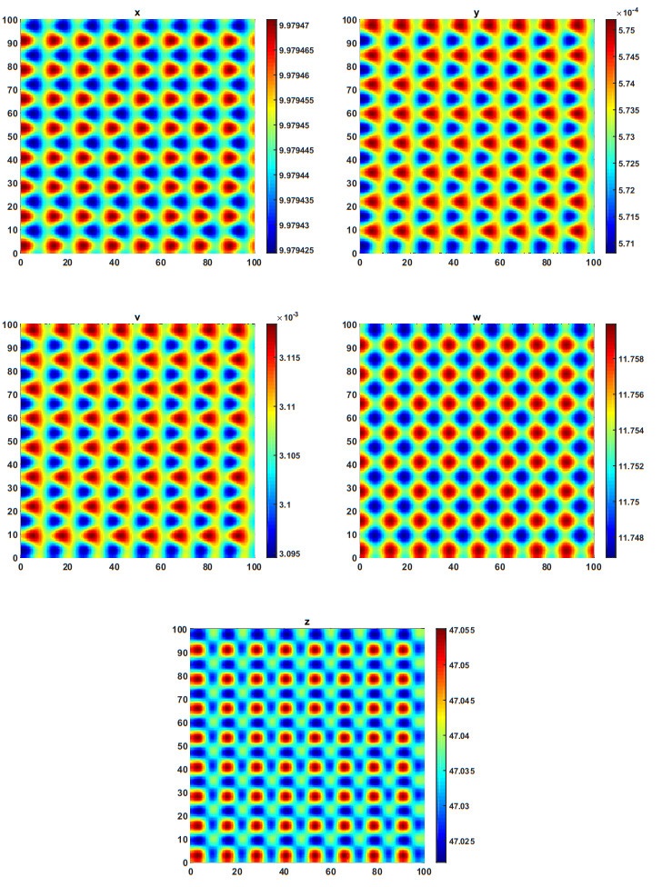
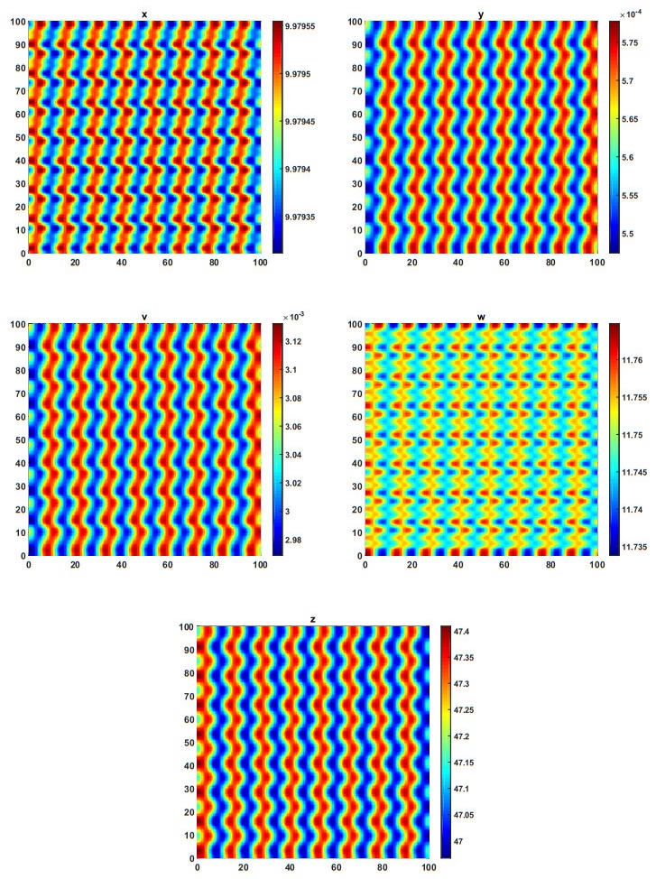
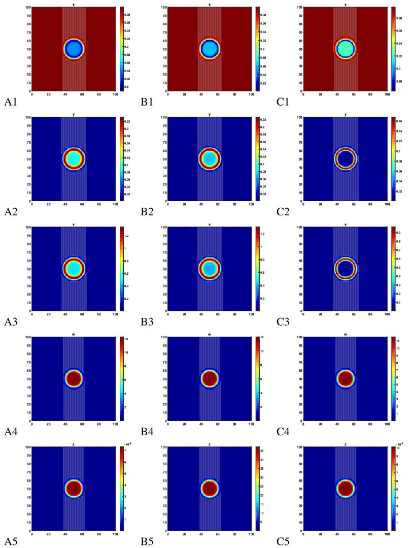
Consistently, influenza has become a major cause of illness and mortality worldwide and it has posed a serious threat to global public health particularly among the immuno-compromised people all around the world. The development of medication to control influenza has become a major challenge now. This work proposes and analyzes a structured model based on two geographical areas, in order to study the spread of influenza. The overall underlying population is separated into two sub populations: urban and rural. This geographical distinction is required as the immunity levels are significantly higher in rural areas as compared to urban areas. Hence, this paper is a novel attempt to proposes a linear and non-linear mathematical model with adaptive immunity and compare the host immune response to disease. For both the models, disease-free equilibrium points are obtained which are locally as well as globally stable if the reproduction number is less than 1 (R01 < 1 & R02 < 1) and the endemic point is stable if the reproduction number is greater then 1 (R01 > 1 & R02 > 1). Next, we have incorporated two treatments in the model that constitute the effectiveness of antidots and vaccination in restraining viral creation and slow down the production of new infections and analyzed an optimal control problem. Further, we have also proposed a spatial model involving diffusion and obtained the local stability for both the models. By the use of local stability, we have derived the Turing instability condition. Finally, all the theoretical results are verified with numerical simulation using MATLAB.
Citation: Mamta Barik, Chetan Swarup, Teekam Singh, Sonali Habbi, Sudipa Chauhan. Dynamical analysis, optimal control and spatial pattern in an influenza model with adaptive immunity in two stratified population[J]. AIMS Mathematics, 2022, 7(4): 4898-4935. doi: 10.3934/math.2022273
Consistently, influenza has become a major cause of illness and mortality worldwide and it has posed a serious threat to global public health particularly among the immuno-compromised people all around the world. The development of medication to control influenza has become a major challenge now. This work proposes and analyzes a structured model based on two geographical areas, in order to study the spread of influenza. The overall underlying population is separated into two sub populations: urban and rural. This geographical distinction is required as the immunity levels are significantly higher in rural areas as compared to urban areas. Hence, this paper is a novel attempt to proposes a linear and non-linear mathematical model with adaptive immunity and compare the host immune response to disease. For both the models, disease-free equilibrium points are obtained which are locally as well as globally stable if the reproduction number is less than 1 (R01 < 1 & R02 < 1) and the endemic point is stable if the reproduction number is greater then 1 (R01 > 1 & R02 > 1). Next, we have incorporated two treatments in the model that constitute the effectiveness of antidots and vaccination in restraining viral creation and slow down the production of new infections and analyzed an optimal control problem. Further, we have also proposed a spatial model involving diffusion and obtained the local stability for both the models. By the use of local stability, we have derived the Turing instability condition. Finally, all the theoretical results are verified with numerical simulation using MATLAB.

| [1] | British Columbia, BC's Pandemic Influenza Response Plan–Introduction and Background, 2012. Available from: https://www2.gov.bc.ca/assets/gov/health/about-bc-s-health-care-system/office-of-the-provincial-health-officer/reports-publications/bc-pandemic-influenza-immunization-response-plan.pdf. |
| [2] |
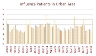
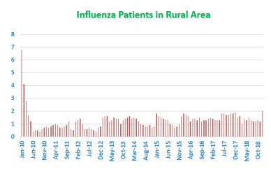
Y. Chen, K. Leng, Y. Lu, L. Wen, Y. Qi, W. Gao, et al., Epidemiological features and time-series analysis of influenza incidence in urban and rural areas of Shenyang, China, 2010–2018, Epidemiol. Infect., 148 (2020), E29. http://dx.doi.org/10.1017/S0950268820000151 doi: 10.1017/S0950268820000151

|
| [3] |
T. S. Böbel, S. B. Hackl, D. Langgartner, M. N. Jarczok, N. Rohleder, C. G. A. Rook, et al., Less immune activation following social stress in rural vs. urban participants raised with regular or no animal contact, respectively, PNAS, 115 (2018), 5259–5264. http://dx.doi.org/10.1073/pnas.1719866115 doi: 10.1073/pnas.1719866115
|
| [4] | N. K. Goswami, B. Shanmukha, A mathematical model of influenza: stability and treatment, Proceedings of the International Conference on Mathematical Modeling and Simulation (ICMMS 16), 2016. |
| [5] |
K. Cheng, P. Leung, What happened in china during the 1918 influenza pandemic?, Int. J. Infect. Dis., 11 (2007), 360–364. http://dx.doi.org/10.1016/j.ijid.2006.07.009 doi: 10.1016/j.ijid.2006.07.009
|
| [6] |
P. R. S. Hastings, D. Krewski, Reviewing the history of pandemic influenza: understanding patterns of emergence and transmission, Pathogens, 5 (2016), 66. http://dx.doi.org/10.3390/pathogens5040066 doi: 10.3390/pathogens5040066
|
| [7] | CDC, Past Pandemics, CDC, Atlanta, GA, USA, 2017. Available from: https://www.cdc.gov/flu/pandemic-resources/basics/past-pandemics.html. |
| [8] |
M. E. Alexander, C. Bowman, S. M. Moghadas, R. Summers, A. B. Gumel, B. M. Sahai, A vaccination model for transmission dynamics of influenza, SIAM J. Appl. Dyn. Syst., 3 (2004), 503–524. http://dx.doi.org/10.1137/030600370 doi: 10.1137/030600370
|
| [9] |
R. Casagrandi, L. Bolzoni, S. A. Levin, V. Andreasen, The SIRC model and influenza A, Math. Biosci., 200 (2006), 152–169. http://dx.doi.org/10.1016/j.mbs.2005.12.029 doi: 10.1016/j.mbs.2005.12.029
|
| [10] |
M. Wille, E. C. Holmes, The ecology and evolution of the influenza viruses, CSH Perspect. Med., 10 (2020), a038489. http://dx.doi.org/10.1101/cshperspect.a038489 doi: 10.1101/cshperspect.a038489
|
| [11] |
H. W. Hethcote, The mathematics of infectious diseases, SIAM Rev., 42 (2000), 599–653. http://dx.doi.org/10.1137/S0036144500371907 doi: 10.1137/S0036144500371907
|
| [12] |
H. Wei, S. Wang, Q. Chen, Y. Chen, X. Chi, L. Zhang, et al., Suppression of interferon lambda signaling by SOCS-1 results in their excessive production during influenza virus infection, PLoS Pathog., 10 (2014), e1003845. http://dx.doi.org/10.1371/journal.ppat.1003845 doi: 10.1371/journal.ppat.1003845
|
| [13] |
J. R. Silveyra, A. R. Mikler, Modeling immune response and its effect on infectious disease outbreak dynamics, Theor. Biol. Med. Model., 13 (2016), 10. http://dx.doi.org/10.1186/s12976-016-0033-6 doi: 10.1186/s12976-016-0033-6
|
| [14] |
H. Y. Lee, D. J. Topham, S. Y. Park, J. Hollenbaugh, J. Treanor, T. R. Mosmann, et al., Simulation and prediction of the adaptive immune response to influenza a virus infection, J. Virol., 83 (2009), 7151–7165. http://dx.doi.org/10.1128/JVI.00098-09 doi: 10.1128/JVI.00098-09
|
| [15] |
J. M. McCaw, J. M. Vernon, Prophylaxis or treatment? Optimal use of an antiviral stockpile during an influenza pandemic, Math. Biosci., 209 (2007), 336–360. http://dx.doi.org/10.1016/j.mbs.2007.02.003 doi: 10.1016/j.mbs.2007.02.003
|
| [16] |
C. W. Kanyiri, K. Mark, L. Luboobi, Mathematical analysis of influenza a dynamics in the emergence of drug resistance, Comput. Math. Method Med., 2018 (2018), 2434560. http://dx.doi.org/10.1155/2018/2434560 doi: 10.1155/2018/2434560
|
| [17] |
C. W. Kanyiri, L. Luboobi, M. Kimathi, Application of optimal control to influenza pneumonia coinfection with antiviral resistance, Comput. Math. Method Med., 2020 (2020), 5984095. http://dx.doi.org/10.1155/2020/5984095 doi: 10.1155/2020/5984095
|
| [18] |
D. M. Weinstock, G. Zuccotti, The evolution of influenza resistance and treatment, JAMA, 301 (2009), 1066–1069. http://dx.doi.org/10.1001/jama.2009.324 doi: 10.1001/jama.2009.324
|
| [19] |
B. Fireman, J. Lee, N. Lewis, O. Bembom, M. van der Laan, R. Baxter, Influenza vaccination and mortality: differentiating vaccine effects from bias, Am. J. Epidemiol., 170 (2009), 650–656. https://doi.org/10.1093/aje/kwp173 doi: 10.1093/aje/kwp173
|
| [20] |
I. G. Barr, J. Mc Cauleyc, N. Cox, R. Daniels, O. G. Engelhardtf, K. Fukuda, et al., Epidemiological, antigenic and genetic characteristics of seasonal influenza A(H1N1), A(H3N2) and B influenza viruses: Basis for the WHO recommendation on the composition of influenza vaccines for use in the 2009–2010 Northern Hemisphere season, Vaccine, 28 (2010), 1156–1167. http://dx.doi.org/10.1016/j.vaccine.2009.11.043 doi: 10.1016/j.vaccine.2009.11.043
|
| [21] | O. Prosper, O. Saucedo, D. Thompson, G. Torres-Garcia, X. Wang, Vaccination strategy and optimal control for seasonal and H1N1 influenza outbreak, 2009. Available from: https://qrlssp.asu.edu/2009-1. |
| [22] | M. Elhia, O. Balatif, J. Bouyaghroumni, E. Labriji, M. Rachik, Optimal control applied to the spread of influenza A(H1N1), Applied Mathematical Sciences, 6 (2012), 4057–4065. |
| [23] | A. K. Srivastav, M. Ghosh, Analysis of a simple influenza A (H1N1) model with optimal control, World Journal of Modelling and Simulation, 12 (2016), 307–319. |
| [24] | S. R. Gani, S. V. Halawar, Deterministic and stochastic optimal control analysis of an SIR epidemic model, Global Journal of Pure and Applied Mathematics, 13 (2017), 5761–5778. |
| [25] |
S. Kim, J. Lee, E. Jung, Mathematical model of transmission dynamics and optimal control strategies for 2009 A/H1N1 influenza in the Republic of Korea, J. Theor. Biol., 9 (2017), 74–85. http://dx.doi.org/10.1016/j.jtbi.2016.09.025 doi: 10.1016/j.jtbi.2016.09.025
|
| [26] |
A. M. Turing, The chemical basis of morphogenesis, Bull. Math. Biol., 52 (1990), 153–197. http://dx.doi.org/10.1007/BF02459572 doi: 10.1007/BF02459572
|
| [27] |
L. A. Segel, J. L. Jackson, Dissipative structure: an explanation and an ecological example, J. Theor. Biol., 37 (1972), 545–559. http://dx.doi.org/10.1016/0022-5193(72)90090-2 doi: 10.1016/0022-5193(72)90090-2
|
| [28] |
T. Singh, S. Banerjee, Spatial aspect of hunting cooperation in predators with Holling type II functional response, J. Biol. Syst., 26 (2018), 511–531. http://dx.doi.org/10.1142/S0218339018500237 doi: 10.1142/S0218339018500237
|
| [29] |
T. Singh, S. Banerjee, Spatiotemporal model of a predator–prey system with herd behavior and quadratic mortality, Int. J. Bifurcat. Chaos, 29 (2019), 1950049. http://dx.doi.org/10.1142/S0218127419500494 doi: 10.1142/S0218127419500494
|
| [30] |
T. Singh, R. Dubey, Spatial patterns dynamics of a diffusive predator-prey system with cooperative behavior in predators, Fractals, 29 (2021), 2150085. http://dx.doi.org/10.1142/S0218348X21500857 doi: 10.1142/S0218348X21500857
|
| [31] |
P. Gulati, S. Chauhan, A. Mubayi, T. Singh, P. Rana, Dynamical analysis, optimum control and pattern formation in the biological pest (EFSB) control model, Chaos Soliton. Fract., 147 (2021), 110920. http://dx.doi.org/10.1016/j.chaos.2021.110920 doi: 10.1016/j.chaos.2021.110920
|
| [32] |
H. E. Jung, H. K. Lee, Host protective immune responses against influenza a virus infection, Viruses, 12 (2020), 504. http://dx.doi:10.3390/v12050504 doi: 10.3390/v12050504
|
| [33] |
A. T. Huang, B. G. Carreras, M. D. T. Hitchings, B. Yang, L. C. Katzelnick, S. M. Rattigan, et al., A systematic review of antibody mediated immunity to coronaviruses: kinetics, correlates of protection, and association with severity, Nature Commun., 11 (2020), 4704. http://dx.doi.org/10.1038/s41467-020-18450-4 doi: 10.1038/s41467-020-18450-4
|
| [34] | M. Nagumo, Uber die Lage der Integralkurven gew onlicher differential gleichungen, Proc. Phys. Math. Soc. Jpn., 24 (1942), 551–559. |
| [35] | G. Birkhoff, G. C. Rota, Ordinary differential equations, New York, NY: Springer, 1982. |
| [36] |
Z. Shuai, P. V. Driessche, Global stability of infectious disease models using Lyapunov functions, SIAM J. Appl. Math., 73 (2013), 1513–1532. http://dx.doi.org/10.1515/msds-2019-0002 doi: 10.1515/msds-2019-0002
|
| [37] |
H. Guo, M. Y. Li, Z. Shuai, A graph-theoretic approach to the method of global Lyapunov functions, Proc. Amer. Math. Soc., 136 (2008), 2793–2802. http://dx.doi.org/10.1090/S0002-9939-08-09341-6 doi: 10.1090/S0002-9939-08-09341-6
|
| [38] |
K. Bessey, M. Mavis, J. Rebaza, J. Zhang, Global stability analysis of a general model of zika virus, Nonauton. Dyn. Syst., 6 (2019), 18–34. http://dx.doi.org/10.1515/msds-2019-0002 doi: 10.1515/msds-2019-0002
|
| [39] | D. L. Lukes, Differential equations: Classical to controlled, New York: Academic Press, 1982. |
| [40] | S. Harroudi, D. Bentaleb, Y. Tabit, S. Amine, K. Allali, Optimal control of an HIV infection model with the adaptive immune response and two saturated rates, Int. J. Math. Comput. Sci., 14 (2019), 787–807. |
| [41] | L. S. Pontryagin, V. G. Boltyanskii, R. V. Gamkrelidze, E. F. Mishchenko, The mathematical theory of optimal processes, New York: John Wiley & Sons, 1962. |
| [42] | W. H. Fleming, R. W. Rishel, Deterministic and stochastic optimal control, New York, NY: Springer, 1975. http://dx.doi.org/10.1007/978-1-4612-6380-7 |
| [43] |
M. Mbow, M. S. E. deJong, L. Meurs, S. Mboup, T. N. Dieye, K. Polman, et al., Changes in immunological profile as a function of urbanization and lifestyle, Immunology, 143 (2014), 569–577. http://dx.doi.org/10.1111/imm.12335 doi: 10.1111/imm.12335
|
| [44] |
E. V. Riet, A. A. Adegnika, K. Retra, R. Vieira, A. G. M. Tielens, B. Lell, et al., Cellular and humoral responses to influenza in gabonese children living in rural and semi-crban areas, The Journal of Infectious Diseases, 196 (2007), 1671–1678. http://dx.doi.org/10.1086/522010 doi: 10.1086/522010
|
Figures(15) / Tables(4)

Mamta Barik, Chetan Swarup, Teekam Singh, Sonali Habbi, Sudipa Chauhan. Dynamical analysis, optimal control and spatial pattern in an influenza model with adaptive immunity in two stratified population[J]. AIMS Mathematics, 2022, 7(4): 4898-4935. doi: 10.3934/math.2022273


 DownLoad: