Analytical solution of time-fractional Schr<i>ö</i>dinger equations via Shehu Adomian Decomposition Method

Mamta Kapoor; Nehad Ali Shah; Wajaree Weera; Mamta Kapoor; Nehad Ali Shah; Wajaree Weera

doi:10.3934/math.20221074

AIMS Mathematics

2022, Volume 7, Issue 10: 19562-19596. doi: 10.3934/math.20221074

Previous Article Next Article

Research article

Analytical solution of time-fractional Schrödinger equations via Shehu Adomian Decomposition Method

1.
Department of Mathematics, Lovely Professional University, Phagwara, Punjab, India
2.
Department of Mechanical Engineering Sejong University, Seoul 05006, South Korea
3.
Department of Mathematics, Faculty of Science, Khon Kaen University, Khon Kaen 40002, Thailand
^†These authors contributed equally to this work and are co-first authors

Received: 29 June 2022 Revised: 27 July 2022 Accepted: 08 August 2022 Published: 05 September 2022
MSC : 49M27, 35R11

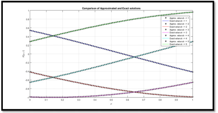
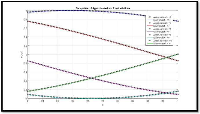
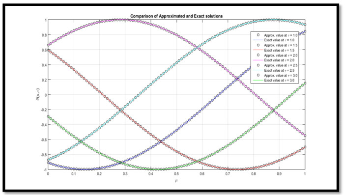
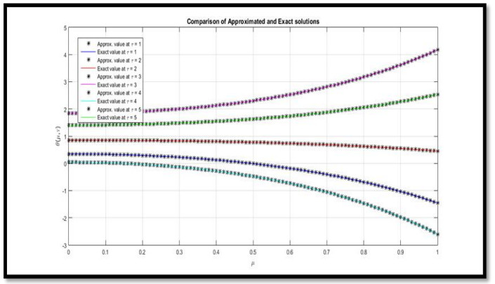
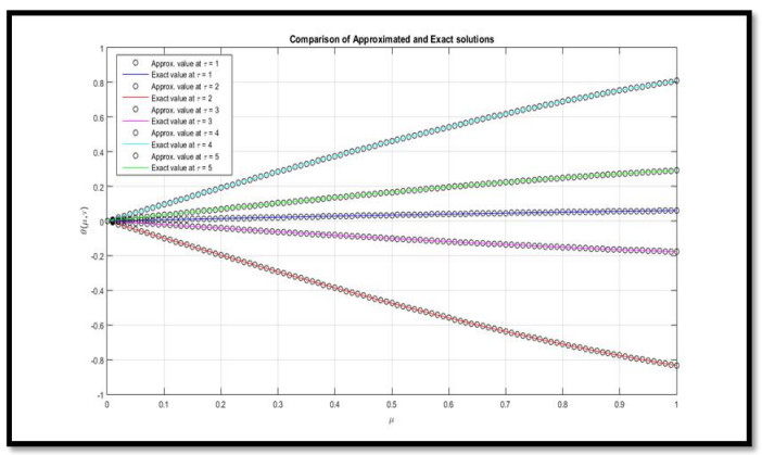
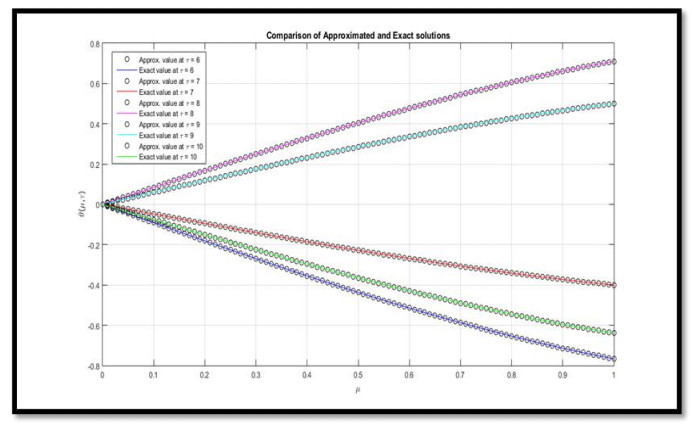
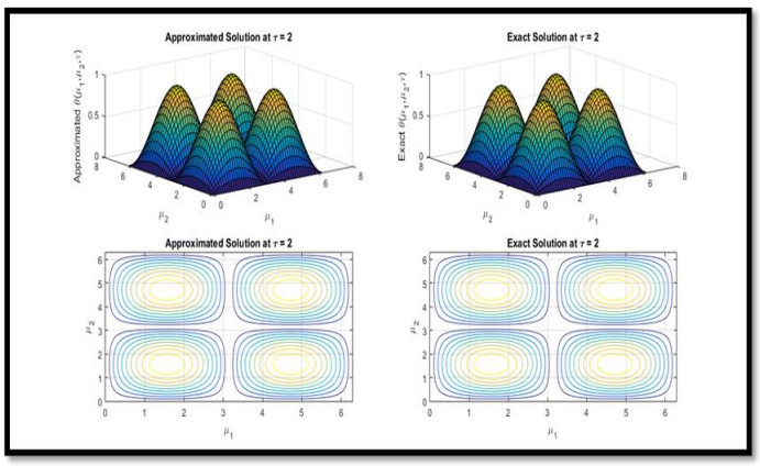
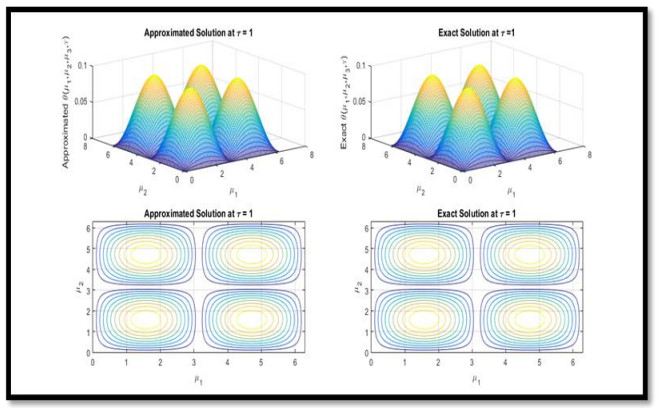
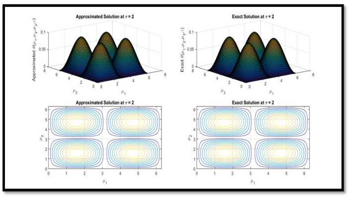
Present research deals with the time-fractional Schrödinger equations aiming for the analytical solution via Shehu Transform based Adomian Decomposition Method [STADM]. Three types of time-fractional Schrödinger equations are tackled in the present research. Shehu transform ADM is incorporated to solve the time-fractional PDE along with the fractional derivative in the Caputo sense. The developed technique is easy to implement for fetching an analytical solution. No discretization or numerical program development is demanded. The present scheme will surely help to find the analytical solution to some complex-natured fractional PDEs as well as integro-differential equations. Convergence of the proposed method is also mentioned.
- time-fractional Schrödinger equations,
- Shehu transform,
- Adomian Decomposition Method,
- graphical presentation,
- tabular analysis,
- convergence property
Citation: Mamta Kapoor, Nehad Ali Shah, Wajaree Weera. Analytical solution of time-fractional Schrödinger equations via Shehu Adomian Decomposition Method[J]. AIMS Mathematics, 2022, 7(10): 19562-19596. doi: 10.3934/math.20221074

Related Papers:

Abstract

Present research deals with the time-fractional Schrödinger equations aiming for the analytical solution via Shehu Transform based Adomian Decomposition Method [STADM]. Three types of time-fractional Schrödinger equations are tackled in the present research. Shehu transform ADM is incorporated to solve the time-fractional PDE along with the fractional derivative in the Caputo sense. The developed technique is easy to implement for fetching an analytical solution. No discretization or numerical program development is demanded. The present scheme will surely help to find the analytical solution to some complex-natured fractional PDEs as well as integro-differential equations. Convergence of the proposed method is also mentioned.

References

[1]	K. Oldham, J. Spanier, The fractional calculus theory and applications of differentiation and integration to arbitrary order, 1 Ed., Elsevier, 1974.
[2]	K. S. Miller, B. Ross, An introduction to the fractional calculus and fractional differential equations, 1 Ed., Wiley, 1993.
[3]	S. G. Samko, A. A. Kilbas, O. I. Marichev, Fractional integrals and derivatives: Theory and applications, USA, 1993.
[4]	I. Podlubny, Fractional differential equations: An introduction to fractional derivatives, fractional differential equations, to methods of their solution and some of their applications, Elsevier, 1998.
[5]	A. A. Kilbas, H. M. Srivastava, J. J. Trujillo, Theory and applications of fractional differential equations, Vol. 204, Elsevier, 2006.
[6]	M. D. Ortigueira, Fractional calculus for scientists and engineers, Vol. 84, Springer Dordrecht, 2011. https://doi.org/10.1007/978-94-007-0747-4
[7]	S. Das, Functional fractional calculus, Springer Berlin, Heidelberg, 2011. https://doi.org/10.1007/978-3-642-20545-3
[8]	R. Hilfer, Applications of fractional calculus in physics, World Scientific, 2000. https://doi.org/10.1142/3779
[9]	B. J. West, M., Bologna, P. Grigolini, Physics of fractal operators, Vol. 35, New York: Springer, 2003. https://doi.org/10.1007/978-0-387-21746-8
[10]	L. Debnath, Recent applications of fractional calculus to science and engineering, Int. J. Math. Math. Sci., 2003 (2003), 3413–3442. https://doi.org/10.1155/S0161171203301486 doi: 10.1155/S0161171203301486
[11]	F. Mainardi, Fractional calculus and waves in linear viscoelasticity: An introduction to mathematical models, World Scientific, 2010. https://doi.org/10.1142/p614
[12]	D. Baleanu, Z. B. Güvenç, J. T. Machado, New trends in nanotechnology and fractional calculus applications, New York: Springer, 2010. https://doi.org/10.1007/978-90-481-3293-5
[13]	R. Herrmann, Fractional calculus: An introduction for physicists, World Scientific, 2011.
[14]	A. Papoulis, A new method of inversion of the Laplace transform, Q. Appl. Math., 14 (1957), 405–414.
[15]	A. Kılıçman, H. E. Gadain, On the applications of Laplace and Sumudu transforms, J. Franklin Inst., 347 (2010), 848–862. https://doi.org/10.1016/j.jfranklin.2010.03.008 doi: 10.1016/j.jfranklin.2010.03.008
[16]	T. M. Elzaki, On the connections between Laplace and Elzaki transforms, Adv. Theor. Appl. Math., 6 (2011), 1–10.
[17]	M. S. Rawashdeh, S. Maitama, Solving coupled system of nonlinear PDE's using the natural decomposition method, Int. J. Pure Appl. Math., 92 (2014), 757–776. https://doi.org/10.12732/ijpam.v92i5.10 doi: 10.12732/ijpam.v92i5.10
[18]	S. Maitama, W. Zhao, New integral transform: Shehu transform a generalization of Sumudu and Laplace transform for solving differential equations, Int. J. Nonlinear Anal. Appl., 17 (2019), 167–190. https://doi.org/10.28924/2291-8639-17-2019-167 doi: 10.28924/2291-8639-17-2019-167
[19]	D. Ziane, R. Belgacem, A. Bokhari, A new modified Adomian decomposition method for nonlinear partial differential equations, Open J. Math. Anal., 3 (2019), 81–90. https://doi.org/10.30538/psrp-oma2019.0041 doi: 10.30538/psrp-oma2019.0041
[20]	L. Akinyemi, O. S. Iyiola, Exact and approximate solutions of time‐fractional models arising from physics via Shehu transform, Math. Methods Appl. Sci., 43 (2020), 7442–7464. https://doi.org/10.1002/mma.6484 doi: 10.1002/mma.6484
[21]	R. Belgacem, D. Baleanu, A. Bokhari, Shehu transform and applications to Caputo-fractional differential equations, Int. J. Anal. Appl., 17 (2019), 917–927. https://doi.org/10.28924/2291-8639-17-2019-917 doi: 10.28924/2291-8639-17-2019-917
[22]	A. K. Shukla, J. C. Prajapati, On a generalization of Mittag-Leffler function and its properties, J. Math. Anal. Appl., 336 (2007), 797–811. https://doi.org/10.1016/j.jmaa.2007.03.018 doi: 10.1016/j.jmaa.2007.03.018
[23]	O. S. Iyiola, E. O. Asante-Asamani, B. A. Wade, A real distinct poles rational approximation of generalized Mittag-Leffler functions and their inverses: Applications to fractional calculus, J. Comput. Appl. Math., 330 (2018), 307–317. https://doi.org/10.1016/j.cam.2017.08.020 doi: 10.1016/j.cam.2017.08.020
[24]	Y. S. Kivshar, G. P. Agrawal, Optical solitons: From fibers to photonic crystals, Academic Press, 2003.
[25]	F. Dalfovo, S. Giorgini, L. P. Pitaevskii, S. Stringari, Theory of Bose-Einstein condensation in trapped gases, Rev. Mod. Phys., 71 (1999), 463. https://doi.org/10.1103/RevModPhys.71.463 doi: 10.1103/RevModPhys.71.463
[26]	J. Belmonte-Beitia, G. F. Calvo, Exact solutions for the quintic nonlinear Schrödinger equation with time and space modulated nonlinearities and potentials, Phys. Lett. A, 373 (2009), 448–453. https://doi.org/10.1016/j.physleta.2008.11.056 doi: 10.1016/j.physleta.2008.11.056
[27]	T. Xu, B. Tian, L. L. Li, X. Lü, C. Zhang, Dynamics of Alfvén solitons in inhomogeneous plasmas, Phys. Plasmas, 15 (2008), 102307. https://doi.org/10.1063/1.2997340 doi: 10.1063/1.2997340
[28]	M. Naber, Time fractional Schrödinger equation, J. Math. Phys., 45 (2004), 3339–3352. https://doi.org/10.1063/1.1769611 doi: 10.1063/1.1769611
[29]	S. Wang, M. Xu, Generalized fractional Schrödinger equation with space-time fractional derivatives, J. Math. Phys., 48 (2007), 043502. https://doi.org/10.1063/1.2716203 doi: 10.1063/1.2716203
[30]	S. Z. Rida, H. M. El-Sherbiny, A. A. M. Arafa, On the solution of the fractional nonlinear Schrödinger equation, Phys. Lett. A, 372 (2008), 553–558. https://doi.org/10.1016/j.physleta.2007.06.071 doi: 10.1016/j.physleta.2007.06.071
[31]	R. K. Saxena, R. Saxena, S. L. Kalla, Computational solution of a fractional generalization of the Schrödinger equation occurring in quantum mechanics, Appl. Math. Comput., 216 (2010), 1412–1417. https://doi.org/10.1016/j.amc.2010.02.041 doi: 10.1016/j.amc.2010.02.041
[32]	J. R. Wang, Y. Zhou, W. Wei, Fractional Schrödinger equations with potential and optimal controls, Nonlinear Anal.: Real World Appl., 13 (2012), 2755–2766. https://doi.org/10.1016/j.nonrwa.2012.04.004 doi: 10.1016/j.nonrwa.2012.04.004
[33]	N. A. Khan, M. Jamil, A. Ara, Approximate solutions to time-fractional Schrödinger equation via homotopy analysis method, Int. Scholarly Res. Not., 2012 (2012), 1–11.
[34]	K. M. Hemida, K. A. Gepreel, M. S. Mohamed, Analytical approximate solution to the time-space nonlinear partial fractional differential equations, Int. J. Pure Appl. Math., 78 (2012), 233–243.
[35]	S. H. M. Hamed, E. A. Yousif, A. I. Arbab, Analytic and approximate solutions of the space-time fractional Schrödinger equations by homotopy perturbation Sumudu transform method, Abstr. Appl. Anal., 2014 (2014), 863015. https://doi.org/10.1155/2014/863015 doi: 10.1155/2014/863015
[36]	S. O. Edeki, G. O. Akinlabi, S. A. Adeosun, Analytic and numerical solutions of time-fractional linear Schrödinger equation, Commun. Math. Appl., 7 (2016), 1–10. https://doi.org/10.26713/cma.v7i1.327 doi: 10.26713/cma.v7i1.327
[37]	A. Mohebbi, M. Abbaszadeh, M. Dehghan, The use of a meshless technique based on collocation and radial basis functions for solving the time fractional nonlinear Schrödinger equation arising in quantum mechanics, Eng. Anal. Boundary Elem., 37 (2013), 475–485. https://doi.org/10.1016/j.enganabound.2012.12.002 doi: 10.1016/j.enganabound.2012.12.002
[38]	K. Shah, M. Junaid, N. Ali, Extraction of Laplace, Sumudu, Fourier and Mellin transform from the natural transform, J. Appl. Environ. Biol. Sci., 5 (2015), 108–115.
[39]	A. N. Malik, O. H. Mohammed, Two efficient methods for solving fractional Lane–Emden equations with conformable fractional derivative, J. Egypt. Math. Soc., 28 (2020), 1–11.
[40]	S. Ali, S. Bushnaq, K. Shah, K. M. Arif, Numerical treatment of fractional order Cauchy reaction diffusion equations, Chaos, Solitons Fract., 103 (2017), 578–587. https://doi.org/10.1016/j.chaos.2017.07.016 doi: 10.1016/j.chaos.2017.07.016
[41]	K. Shah, H. Naz, M. Sarwar, T. Abdeljawad, On spectral numerical method for variable-order partial differential equations, AIMS Math., 7 (2022), 10422–10438. https://doi.org/10.3934/math.2022581 doi: 10.3934/math.2022581
[42]	A. Bashan, N. M. Yagmurlu, Y. Ucar, A. Esen, An effective approach to numerical soliton solutions for the Schrödinger equation via modified cubic B-spline differential quadrature method, Chaos, Solitons Fract., 100 (2017), 45–56. https://doi.org/10.1016/j.chaos.2017.04.038 doi: 10.1016/j.chaos.2017.04.038
[43]	N. A. Shah, P. Agarwal, J. D. Chung, E. R. El-Zahar, Y. S. Hamed, Analysis of optical solitons for nonlinear Schrödinger equation with detuning term by iterative transform method, Symmetry, 12 (2020), 1850. https://doi.org/10.3390/sym12111850 doi: 10.3390/sym12111850
[44]	N. A. Shah, I. Dassios, E. R. El-Zahar, J. D. Chung, S. Taherifar, The variational iteration transform method for solving the time-fractional Fornberg-Whitham equation and comparison with decomposition transform method, Mathematics, 9 (2021), 141. https://doi.org/10.3390/math9020141 doi: 10.3390/math9020141
[45]	M. Kapoor, N. A. Shah, S. Saleem, W. Weera, An analytical approach for fractional hyperbolic telegraph equation using Shehu transform in one, two and three dimensions, Mathematics, 10 (2022), 1961. https://doi.org/10.3390/math10121961 doi: 10.3390/math10121961
[46]	M. Kapoor, A. Majumder, V. Joshi, An analytical approach for Shehu transform on fractional coupled 1D, 2D and 3D Burgers' equations, Nonlinear Eng., 11 (2022), 268–297. https://doi.org/10.1515/nleng-2022-0024 doi: 10.1515/nleng-2022-0024
[47]	M. Kapoor, Sumudu transform HPM for Klein-Gordon and Sine-Gordon equations in one dimension from an analytical aspect, J. Math. Comput. Sci., 12 (2022), 1–25. https://doi.org/10.28919/jmcs/6979 doi: 10.28919/jmcs/6979

Reader Comments

Your name:*

Email:*
© 2022 the Author(s), licensee AIMS Press. This is an open access article distributed under the terms of the Creative Commons Attribution License (http://creativecommons.org/licenses/by/4.0)