Segmentation-clock synchronization in circular-lattice networks of embryonic presomitic-mesoderm cells

Jesús Pantoja-Hernández; Moisés Santillán; Jesús Pantoja-Hernández; Moisés Santillán

doi:10.3934/math.2021344

AIMS Mathematics

2021, Volume 6, Issue 6: 5817-5836. doi: 10.3934/math.2021344

Previous Article Next Article

Research article Special Issues

Segmentation-clock synchronization in circular-lattice networks of embryonic presomitic-mesoderm cells

Centro de Investigación y de Estudios Avanzados del IPN, Unidad Monterrey, Vía del Conocimiento 201, Parque PIIT, 66628 Apodaca NL, MÉXICO

Received: 02 October 2020 Accepted: 27 February 2021 Published: 26 March 2021
MSC : 37N25, 92B25

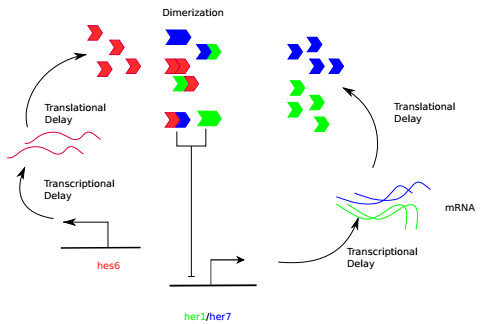
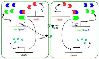
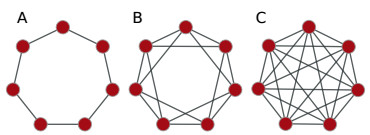
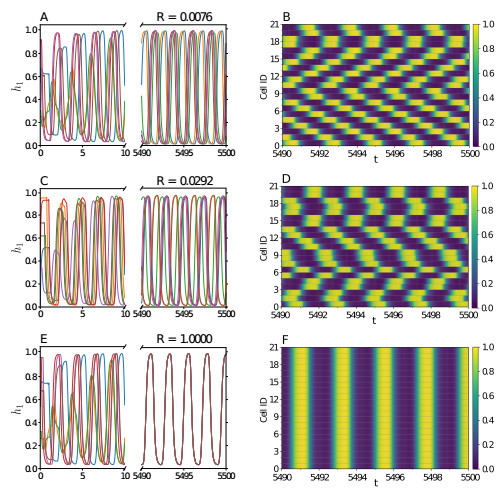
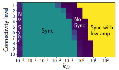
Somitogenesis is the process by means of which a tissue known as presomitic mesoderm (PSM) is segmented in blocks of cells, called somites, along the anterior-posterior axis of the developing embryo in segmented animals. In vertebrates, somites give rise to axial skeleton, cartilage, tendons, skeletal muscle, and dermis. Somite formation occurs periodically, and this periodicity is driven by a genetic oscillator that operates within PSM cells and is known as the segmentation clock. The correct synchronization of the segmentation clock among PSM cells is essential for somitogenesis to develop normally. When synchronization is disrupted, somites form irregularly and, in consequence, the tissues that originate from them show clear malformations. In this work, based in a model for zebrafish segmentation clock, we investigate by means of a mathematical modeling approach, how PSM-cell synchronization is affected by factors like: the size of PSM-cell networks, the amount of cell-to-cell interactions per PSM cell, the strength of these interactions, and the inherent variability among PSM cells. Interestingly we found that very small PSM-cell networks are unable to synchronize. Moreover, the effect of decreasing the strength of interactions among PSM cells is corrected by increasing the network connectivity-level, and a moderated level of variability among cells can have a positive effect on synchronization, specially in large networks.

Keywords:

Citation: Jesús Pantoja-Hernández, Moisés Santillán. Segmentation-clock synchronization in circular-lattice networks of embryonic presomitic-mesoderm cells[J]. AIMS Mathematics, 2021, 6(6): 5817-5836. doi: 10.3934/math.2021344

Related Papers:

[1]	Hongyan Dui, Yong Yang, Xiao Wang . Reliability analysis and recovery measure of an urban water network. Electronic Research Archive, 2023, 31(11): 6725-6745. doi: 10.3934/era.2023339
[2]	Xu Zhan, Yang Yong, Wang Xiao . Phased mission reliability analysis of unmanned ship systems. Electronic Research Archive, 2023, 31(10): 6425-6444. doi: 10.3934/era.2023325
[3]	Majed Alowaidi, Sunil Kumar Sharma, Abdullah AlEnizi, Shivam Bhardwaj . Integrating artificial intelligence in cyber security for cyber-physical systems. Electronic Research Archive, 2023, 31(4): 1876-1896. doi: 10.3934/era.2023097
[4]	Xiaoyang Xie, Shanghua Wen, Minglong Li, Yong Yang, Songru Zhang, Zhiwei Chen, Xiaoke Zhang, Hongyan Dui . Resilience evaluation and optimization for an air-ground cooperative network. Electronic Research Archive, 2024, 32(5): 3316-3333. doi: 10.3934/era.2024153
[5]	Shuang Yao, Dawei Zhang . A blockchain-based privacy-preserving transaction scheme with public verification and reliable audit. Electronic Research Archive, 2023, 31(2): 729-753. doi: 10.3934/era.2023036
[6]	Shanpu Gao, Yubo Li, Anping Wu, Hao Jiang, Feng Liu, Xinlong Feng . An intelligent optimization method for accelerating physical quantity reconstruction in computational fluid dynamics. Electronic Research Archive, 2025, 33(5): 2881-2924. doi: 10.3934/era.2025127
[7]	Wanxun Jia, Ling Li, Haoyan Zhang, Gengxiang Wang, Yang Liu . A novel nonlinear viscous contact model with a Newtonian fluid-filled dashpot applied for impact behavior in particle systems. Electronic Research Archive, 2025, 33(5): 3135-3157. doi: 10.3934/era.2025137
[8]	Sida Lin, Jinlong Yuan, Zichao Liu, Tao Zhou, An Li, Chuanye Gu, Kuikui Gao, Jun Xie . Distributionally robust parameter estimation for nonlinear fed-batch switched time-delay system with moment constraints of uncertain measured output data. Electronic Research Archive, 2024, 32(10): 5889-5913. doi: 10.3934/era.2024272
[9]	Yunying Huang, Wenlin Gui, Yixin Jiang, Fengyi Zhu . Types of systemic risk and macroeconomic forecast: Evidence from China. Electronic Research Archive, 2022, 30(12): 4469-4492. doi: 10.3934/era.2022227
[10]	Yazhou Chen, Dehua Wang, Rongfang Zhang . On mathematical analysis of complex fluids in active hydrodynamics. Electronic Research Archive, 2021, 29(6): 3817-3832. doi: 10.3934/era.2021063

Abstract

1. Introduction

Let $q$ be a power of odd prime. Several researchers have looked into a variety of properties about the primitive roots modulo $q$ . Let $g_1, g_2$ represent two primitive roots modulo $q$ , $a$ , $b$ and $c$ represent arbitrary non-zero elements in $\mathbb{F}_q$ . Is there some $q_0$ such that for all $q > q_0$ , there is always one representation

$\begin{eqnarray} a = bg_1+cg_2\ ? \end{eqnarray}$

(1.1)

For $b = 1$ and $c = -1$ , Vegh ^[1] considered a specific form of Eq (1.1), which is known as Vegh's Conjecture, (see [,§ F9] for further details). Cohen ^[3] demonstrated Vegh's Conjecture for all $q > 7$ .

For $b = 1$ and $c = 1$ , Golomb ^[4] proposed another specific form of Eq (1.1). This was proved by Sun ^[5] for $q > 2^{60}\approx 1.15\times 10^{18}$ .

Moreover, Cohen et al. ^[6] studied linear sums of primitive roots and their inverses in finite fields $\mathbb{F}_q$ and showed that if $q > 13$ , then for arbitrary non-zero $a, b \in \mathbb{F}_q$ , there is a pair of primitive elements ( $g_1$ , $g_2$ ) of $\mathbb{F}_q$ such that both $ag_1+bg_2$ and $ag^{-1}_1+bg^{-1}_2$ are primitive.

Let $p$ be an odd prime. Carlitz ^[7] relied on some results of Davenport and obtained for any $k-1$ fixed integers $c_1, c_2, \ldots, c_{k-1}$ with $c_i \geq 1 (i = 1, 2, \ldots, k-1)$ . Let $g, g_1, \ldots, g_{k-1}$ be primitive roots modulo $p$ and $N_k$ denote the number of $g\bmod p$ such that $g_1-g = c_1, \ldots, g_{k-1}-g = c_{k-1}$ . Then

$\begin{eqnarray*} N_k \sim \frac{\phi^{k}(p-1)}{p^{k-1}}\ \hfill (p\rightarrow \infty). \end{eqnarray*}$

More results of the primitive roots distribution can be found in ^[8,9,10,11].

Lehmer [,§ F12] proposed the definition of $Lehmer~~ number$ , according to which $a$ is a $Lehmer ~~number$ if and only if $a$ and $\bar{a}$ have opposite parity, i.e., $(2, a+\bar{a}) = 1$ , where $\bar{a}$ is the multiplicative inverse of $a$ modulo $p$ . It is simple to demonstrate that there are no Lehmer numbers modulo $p$ when $p = 3$ or $7$ . Zhang ^[12] established that if $M_p$ denotes the number of Lehmer numbers modulo $p$ , then

$\begin{eqnarray*} M_p = \frac{p-1}{2}+\mathrm{O}\left(p^{\frac{1}{2}}\ln^2p\right). \end{eqnarray*}$

A Lehmer number that is also a primitive root modulo $p$ will be called a $Lehmer~~ primitive~~ root$ or an $LPR$ . The inverse of an $LPR$ is also an $LPR$ . We assume that $p > 3$ because there is no Lehmer number modulo $3$ . Wang and Wang ^[13] investigated the distribution of $LPRs$ involving Golomb's conjecture. Let $G_p$ denote the number of Golomb pairs $(a, b)$ (i.e., $a+b\equiv 1(\bmod\; p)$ ) are $LPRs$ . They showed

$\begin{eqnarray*} G_p = \frac{1}{4}\frac{\phi^2(p-1)}{p-1}+O\left(\frac{\phi^2(p-1)}{p^{\frac{5}{4}}}\cdot 4^{\omega(p-1)}\cdot \ln^2p\right). \end{eqnarray*}$

Let $N_p$ denote the number of $LPRs$ modulo $p$ . For odd integers $m\geq 3$ , define the positive number $T_m$ by

$\begin{eqnarray*} T_m = \frac{2}{m\ln m}\sum\limits_{j = 1}^{(m-1)/2}\tan\left(\frac{\pi j}{m}\right). \end{eqnarray*}$

Cohen and Trudgian ^[14] improved the result of Wang and Wang ^[13] and showed

$\begin{eqnarray*} \left|N_p-\frac{\phi(p-1)}{2}\right| < T_p^2\frac{\phi(p-1)}{p-1}2^{\omega(p-1)}p^{\frac{1}{2}}\ln^2p \end{eqnarray*}$

and

$\begin{eqnarray*} \left|G_p-\frac{\phi^2(p-1)}{4(p-1)^2}(p-2)\right| < \frac{\phi^2(p-1)}{4(p-1)^2}T_p^2[2^{2\omega(p-1)}(9\ln^2p+1)-1]p^{\frac{1}{2}}, \end{eqnarray*}$

where $\frac{2}{\pi}\left(1+\frac{0.548}{\ln p}\right) < T_p < \frac{2}{\pi}\left(1+\frac{1.549}{\ln p}\right)$ .

Specifically, they obtained that for an odd prime $p(\neq 3, 7)$ , there exists an $LPR$ modulo $p$ .

Inspired by the results of Cohen and Trudgian ^[14] and Wang and Wang ^[13], we mainly studied the distribution of $LPRs$ modulo $p$ related to the Golomb's conjecture in two aspects. On the one hand, we extend Eq (1.1) to the case involving $k > 1$ variables. Let $\mathcal{R}$ be set of $LPRs$ modulo $p$ that is a subset of ${\mathbb{F}}_p$ . $a_1, a_2, \ldots, a_k, c$ are non-zero elements in ${\mathbb{F}}_p$ and $N(\mathcal{R}, p)$ denotes the number of solutions of the equation

$\begin{eqnarray*} a_1g_1+a_2g_2+\cdots+a_kg_k = c, \ g_1, g_2, \ldots, g_k \in \mathcal{R}. \end{eqnarray*}$

We consider the distribution properties of $N(\mathcal{R}, p)$ , and obtain the following:

Theorem 1. Let $p > 3$ be an odd prime. Then we have

$\begin{eqnarray*} N(\mathcal{R}, p) = \frac{\phi^k(p-1)}{2^kp}+\mathrm{O}\left(\frac{\phi^k(p-1)}{p^\frac{3}{2}}2^{k\omega(p-1)}\ln^{2k}p\right), \end{eqnarray*}$

where the symbol $\mathrm{O}$ is dependent on $k$ .

When $k = 2$ , we can obtain the number of the Golomb pairs that are $LPRs$ .

On the other hand, we consider the distribution of $k$ consecutive $LPRs$ and generalize it to a more general form.

Let $f(x)\in \mathbb{F}_p[x]$ . Define

$\begin{eqnarray*} M(f(x), \mathcal{R}, p) = \#\{x: 1\leq x\leq p-1, f(x+c_1), f(x+c_2), \cdots, f(x+c_k) \in \mathcal{R} \}. \end{eqnarray*}$

Then we have:

Theorem 2. Let $f(x)\in \mathbb{F}_p[x]$ with degree $l\geq 1$ . $c_1, c_2, \ldots, c_k$ are distinct elements in $\mathbb{F}_p$ . Suppose that one of the following conditions holds:

$\rm (i)$ $f(x)$ is irreducible,

$\rm (ii)$ $f(x)$ has no multiple zero in $\bar{\mathbb{F}}_p$ and $k = 2$ ,

$\rm (iii)$ $f(x)$ has no multiple zero in $\bar{\mathbb{F}}_p$ and $(4k)^{l} < p$ .

Then we have

$\begin{eqnarray*} &&M(f(x), \mathcal{R}, p) = \frac{1}{2^k}\frac{\phi^k(p-1)}{(p-1)^{k-1}}+\mathrm{O}\left(\frac{\phi^k(p-1)}{p^{k-\frac{1}{2}}}2^{k\omega(p-1)}\ln^{2k}p\right), \end{eqnarray*}$

where the symbol $\mathrm{O}$ is dependent on $k$ and $l$ .

Take $f(x) = x$ , $c_k = 0$ in Theorem 2. Then we can get the number of $k$ consecutive primitive roots $x, x+c_1, \ldots, x+c_{k-1}$ are Lehmer numbers, which is:

Corollary 1. Let $p$ be an odd prime. Then for any $1\leq\ x\leq(p-1)$ that is an LPR modulo $p$ , we have

$\begin{eqnarray*} &&M(x, \mathcal{R}, p) = \frac{1}{2^k}\frac{\phi^k(p-1)}{(p-1)^{k-1}}+\mathrm{O}\left(\frac{\phi^k(p-1)}{p^{k-\frac{1}{2}}}2^{k\omega(p-1)}\ln^{2k}p\right), \end{eqnarray*}$

where the symbol $\mathrm{O}$ is dependent on $k$ .

When $k = 1, 2$ , we can easily deduce the Theorem 1 and Theorem 6 in Cohen and Trudgian ^[14], respectively.

Notation: Throughout this paper, $\mathbb{F}_q$ denotes a finite field of characteristic $p$ , $\bar{\mathbb{F}}_q$ denotes the algebraic closure of $\mathbb{F}_q$ , $\phi(n)$ is reserved for the Euler function, $\mu(n)$ is the M $\ddot{o}$ bius function. We use $\omega(n)$ to denote the number of all distinct prime divisors of $n$ . Write $\sum_{\chi_d}$ to denote a sum over all $\phi(d)$ multiplicative characters $\chi_d$ of order $d$ over ${\mathbb{F}}_p$ , and denote by $\mathop{\sum_{n = 1}^{p}}^{'}$ the summation of $1\leq n\leq p$ with $(n, p) = 1$ . $\tau(\chi)$ is the classical Gauss sums associated with character $\chi$ mudulo $p$ . $f\ll g$ means $|f|\leq cg$ with some positive constant $c$ , $f = \mathrm{O}(g)$ means $f\ll g$ .

2. Some lemmas

To complete the proof of the theorems, we need following several lemmas. The proofs of these lemmas require some basic knowledge of analytic number theory, which can be found in ^[15].

Lemma 1. Let $p$ be an odd prime. Then for any integer $a$ coprime to $p$ (i.e., $(a, p) = 1$ ), we have the identity

$\frac{\phi(p-1)}{p-1}\sum\limits_{d\mid p-1}\frac{\mu(d)}{\phi(d)}\sum\limits_{\chi_d}\chi_d(a) = \left\{ \begin{array}{ll} 1, &\ { if~~ a ~~ is ~~ a~~ primitive ~~ root ~~ \text{mod}~~ p;}\\ 0, &\ {if~~ a ~~ is~~ not~~ a~~ primitive~~ root~~ \text{mod}~~ p.} \end{array}\right.$

Proof. See Proposition 2.2 of Narkiewicz ^[16]. □

Lemma 2. Let $p$ be an odd prime, $\chi$ be a nonprincipal multiplicative character modulo $p$ of order $d$ . Suppose $g(x)\in \mathbb{F}_p[x]$ has precisely $m$ distinct ones among its zeros, and suppose that $g(x)$ is not the constant multiple of a $d$ -th power over $\mathbb{F}_q$ . Then

$\left|\sum\limits_{x\in \mathbb{F}_p}\chi\left(g(x)\right)\right|\leq \left(m-1\right)\cdot p^{\frac{1}{2}}.$

Proof. See Theorem 2C in Chapter 2 of Schmidt ^[17]. □

Lemma 3. Let $\mathbb{F}_q$ be a finite field of characteristic $p$ , $\psi$ be a nontrivial additive character and $\chi$ be a nonprincipal multiplicative character on $\mathbb{F}_q$ of order $d$ . For two rational functions $f(x), g(x)\in\mathbb{F}_q[x]$ , define $K(\psi, f;\chi, g) = \sum_{x\in\mathbb{F}_q\backslash S}\chi(g(x))\psi(f(x))$ , where $S$ denotes the set of poles of $f(x)$ and $g(x)$ . Suppose the following conditions hold:

$\rm (i)$ $g(x)$ is not the constant multiple of a $d$ -th power over $\mathbb{F}_q$ .

$\rm (ii)$ $f(x)$ is not of the form $(h(x))^p-h(x)$ with a rational function $h(x)$ over $\mathbb{F}_q$ .

Then we have

$|K(\psi, f;\chi, g)|\leq(\deg(f)+m-1)\sqrt{q},$

where $m$ is the number of distinct roots and (noninfinite) poles of $g(x)$ in $\mathbb{F}_q$ .

Proof. See Theorem 2G in Chapter 2 of Schmidt ^[17]. □

Lemma 4. Let $p$ be an odd prime. Let $c_1, \cdots, c_k$ be distinct elements in $\mathbb{F}_p$ . Assume that $f(x)\in\mathbb{F}_{p}[x]$ with $\deg(f) = l$ . Define the polynomial

$h(x) = f(x+c_1)\cdots f(x+c_k).$

Suppose one of the following conditions holds:

$\rm (i)$ $f(x)$ is irreducible,

$\rm (ii)$ $f(x)$ has no multiple zero in $\bar{\mathbb{F}}_p$ and $k = 2$ ,

$\rm (iii)$ $f(x)$ has no multiple zero in $\bar{\mathbb{F}}_p$ and $(4k)^{l} < p$ .

Then $h(x)$ has at least one simple root in $\bar{\mathbb{F}}_p$ .

Proof. Suppose that $f(x)$ is irreducible. Then $f(x+c_1), \cdots, f(x+c_k)$ are distinct irreducible polynomials, and $h(x)$ has at least $k$ simple roots in $\bar{\mathbb{F}}_p$ . The cases of $\rm (ii)$ and $\rm (iii)$ can be proved by Theorem 2 and Lemma 2 of ^[18], for $k = 2$ or $(4k)^{l} < p$ , $(l, k, p)$ is "admissible triple, " then $f(x+c_1)\cdots f(x+c_k)$ has at least one simple root. □

Lemma 5. Let $p$ be an odd prime, $m_1, \ldots, m_k, n_1, \ldots, n_k$ be integers with $(m_1\cdots m_kn_1\cdots n_k, p) = 1$ , and polynomials $g(x), f_1(x), \ldots, f_k(x)\in\mathbb{F}_p[x]$ . Let $\chi$ be a Dirichlet character modulo $p$ of order $d$ . Define

$\begin{eqnarray*} &&K(\chi, g, f_1, \cdots, f_k;p)\\ && = \mathop{\sum\limits_{x = 1}^{p}}_{(f_1(x)\cdots f_k(x), p) = 1}\chi(g(x)) e\left(\frac{m_1f_1(x)+\cdots+m_kf_k(x)+n_1\overline{f_1(x)}+\cdots+n_k\overline{f_k(x)}}{p}\right). \end{eqnarray*}$

Suppose the following conditions hold:

$\rm (i)$ $g(x)$ can not be the constant multiple of a $d$ -th power over $\mathbb{F}_p$ .

$\rm (ii)$ $F(x) = f_1(x)\cdots f_k(x)$ has at least one simple root in $\bar{\mathbb{F}}_p$ .

Then we have

$\begin{eqnarray*} |K(\chi, g, f_1, \cdots, f_k;p)| \leq\left(\max(\deg(f_1), \cdots, \deg(f_k))+l\right)\sqrt{p}, \end{eqnarray*}$

where $e(x) = e^{2\pi ix}$ and $l$ is the number of distinct roots of $g(x)$ in $\bar{\mathbb{F}}_p$ .

Proof. It is clear that

$\begin{eqnarray*} &&m_1f_1(x)+\cdots+m_kf_k(x)+n_1\overline{f_1(x)}+\cdots+n_k\overline{f_k(x)}\\ && = \frac{F(x)(m_1f_1(x)+\cdots+m_kf_k(x))+n_1\frac{F(x)}{f_1(x)}+\cdots +n_k\frac{F(x)}{f_k(x)}}{F(x)} : = \frac{G(x)}{F(x)}. \end{eqnarray*}$

Condition $\rm (i)$ is the same as Lemma 3. So our goal is to prove the rational function $G(x)/F(x)$ satisfies condition $\rm (ii)$ in Lemma 3 if $F(x)$ has a simple root in $\bar{\mathbb{F}}_p$ . Assume that there are polynomials $K(x), L(x)\in\mathbb{F}_p[x]$ with $(K(x), L(x)) = 1$ such that

$\frac{G(x)}{F(x)} = \left(\frac{K(x)}{L(x)}\right)^p-\left(\frac{K(x)}{L(x)}\right).$

Then we have

$\begin{eqnarray} G(x)L(x)^p = \left(K(x)^p-K(x)L(x)^{p-1}\right)F(x). \end{eqnarray}$

(2.1)

Since $F(x) = f_1(x)\cdots f_k(x)$ has at least one simple root in $\bar{\mathbb{F}}_p$ , then there exists an irreducible polynomial $w(x)\in\mathbb{F}_p[x]$ such that $w(x)\mid F(x)$ and $w(x)^2\nmid F(x)$ . Assume that $w(x)\mid f_1(x)$ , then we have

$w(x)\nmid\frac{F(x)}{f_1(x)}, \ w(x)\mid\frac{F(x)}{f_i(x)}(i = 2, \cdots, k).$

Hence, from Eq (2.1)

$w(x)\nmid G(x)\Longrightarrow w(x)\mid L(x)^p\Longrightarrow w(x)\mid L(x)$

$w(x)^2\mid L(x)^{p-1}\Longrightarrow w(x)^2\mid K(x)^pF(x)\Longrightarrow w(x)\mid K(x),$

which contradicts to $(K(x), L(x)) = 1$ . Therefore, from Lemma 3 we get

$\begin{eqnarray*} |K(\chi, g, f_1, \cdots, f_k;p)| \leq\left(\max(\deg(f_1), \cdots, \deg(f_k))+l\right)\sqrt{p}, \end{eqnarray*}$

where $l$ is the number of distinct roots of $g(x)$ in $\bar{\mathbb{F}}_p$ . □

Lemma 6. Let $\chi$ be a primitive character modulo $p$ , $\chi_{d_i}$ be character modulo $p$ of order $d_i$ . There exist some $1\leq s_i\leq d_i$ with $(s_i, d_i) = 1$ , $i = 1, 2, \ldots, k$ . Then we have

Proof. From the definition of the Dirichlet character modulo $p$ , we can get

$\begin{eqnarray*} &&\sum\limits_{\chi_{d_1}}\cdots \sum\limits_{\chi_{d_k}}\chi_{d_1}(f(x+c_1))\cdots \chi_{d_k}(f(x+c_k))\\ & = &\mathop{{\sum\limits_{s_1 = 1}^{d_1}}\ '}\cdots \mathop{{\sum\limits_{s_k = 1}^{d_k}}\ '} e\left(\frac{s_1\cdot \text{ind}(f(x+c_1))}{d_1}\right)\cdots e\left(\frac{s_k\cdot \text{ind}(f(x+c_k))}{d_k}\right)\\ & = &\mathop{{\sum\limits_{s_1 = 1}^{d_1}}\ '}\cdots \mathop{{\sum\limits_{s_k = 1}^{d_k}}\ '}e\left(\frac{\frac{s_1(p-1)}{d_1}\cdot \text{ind}(f(x+c_1))+\cdots+\frac{s_k(p-1)}{d_k}\cdot \text{ind}(f(x+c_k))}{p-1}\right)\\ & = &\mathop{{\sum\limits_{s_1 = 1}^{d_1}}\ '}\cdots \mathop{{\sum\limits_{s_k = 1}^{d_k}}\ '}e\left(\frac{ \text{ind}(f(x+c_1))^{\frac{s_1(p-1)}{d_1}}+\cdots+ \text{ind}(f(x+c_k))^{\frac{s_k(p-1)}{d_k}}}{p-1}\right)\\ & = &\mathop{{\sum\limits_{s_1 = 1}^{d_1}}\ '}\cdots \mathop{{\sum\limits_{s_k = 1}^{d_k}}\ '}e\left(\frac{ \text{ind}\left((f(x+c_1))^{\frac{s_1(p-1)}{d_1}}\cdots(f(x+c_k))^{\frac{s_k(p-1)}{d_k}}\right)}{p-1}\right)\\ & = &\mathop{{\sum\limits_{s_1 = 1}^{d_1}}\ '}\cdots \mathop{{\sum\limits_{s_k = 1}^{d_k}}\ '}\chi\left(f(x+c_1))^{\frac{s_1(p-1)}{d_1}}\cdots(f(x+c_k))^{\frac{s_k(p-1)}{d_k}}\right), \end{eqnarray*}$

where $\text{ind}(a)$ denotes an index of $a$ with base $g$ of modulo $p$ , and $g$ is a positive primitive root of modulo $p$ . □

3. Proofs of the theorems

Firstly, we prove the Theorem 1. Let $p$ be an odd prime, $k$ be any fixed positive integer. Then for any $k$ different integers $a_1, \ a_2, \ldots, a_k \in {\mathbb{F}}_p$ , from Lemma 1 and the definition of Lehmer number we have

$\begin{eqnarray} &&N(\mathcal{R}, p) = \frac{1}{p}\sum\limits_{b = 0}^{p-1}\mathop{\sum\limits_{g_1 = 1}^{p-1}\sum\limits_{g_2 = 1}^{p-1}\cdots \sum\limits_{g_k = 1}^{p-1}}_{g_1, g_2, \ldots, g_k \in \mathcal{R}}e\left(\frac{b(a_1g_1+\cdots+a_kg_k-c)}{p}\right)\\ & = &\frac{1}{p}\frac{\phi^k(p-1)}{2^k(p-1)^k}\prod\limits_{i = 1}^{k}\left(\sum\limits_{d_i\mid p-1}\frac{\mu\left(d_i\right)}{\phi\left(d_i\right)}\sum\limits_{\chi_{d_i}}\sum\limits_{g_i = 1}^{p-1} \chi_{d_i}(g_i)\left(1-(-1)^{g_i+\overline{g_i}}\right)\right)\\ &&\cdot \sum\limits_{b = 0}^{p-1}e\left(\frac{b(a_1g_1+\cdots+a_kg_k-c)}{p}\right)\\ & = &\frac{1}{p}\frac{\phi^k(p-1)}{2^k(p-1)^k}\prod\limits_{i = 1}^{k}\left(\sum\limits_{d_i\mid p-1}\frac{\mu\left(d_i\right)}{\phi\left(d_i\right)}\sum\limits_{\chi_{d_i}}\sum\limits_{g_i = 1}^{p-1} \chi_{d_i}(g_i)\right)\sum\limits_{b = 0}^{p-1}e\left(\frac{b(a_1g_1+\cdots+a_kg_k-c)}{p}\right)\\ &&+\frac{1}{p}\frac{\phi^k(p-1)}{2^k(p-1)^k}\prod\limits_{i = 1}^{k}\left(\sum\limits_{d_i\mid p-1}\frac{\mu\left(d_i\right)}{\phi\left(d_i\right)}\sum\limits_{\chi_{d_i}}\sum\limits_{g_i = 1}^{p-1} \chi_{d_i}(g_i)\right)\sum\limits_{t = 1}^{k}(-1)^{t}\mathop{\sum\limits_{i_1 = 1}^{k}\sum\limits_{i_2 = 1}^{k}\cdots \sum\limits_{i_t = 1}^{k}}_{i_1 < i_2 < \cdots < i_t}l_{i_1}l_{i_2}\cdots l_{i_t}\\ &&\cdot \sum\limits_{b = 0}^{p-1}e\left(\frac{b(a_1g_1+\cdots+a_kg_k-c)}{p}\right)\\ & = &A_1+A_2, \end{eqnarray}$

(3.1)

where $l_i = (-1)^{g_i+\overline{g_i}}, i = 1, 2, \cdots, k$ .

$\begin{eqnarray} &&A_1 = \frac{1}{p}\frac{\phi^k(p-1)}{2^k(p-1)^k}\prod\limits_{i = 1}^{k}\left(\sum\limits_{d_i\mid p-1}\frac{\mu\left(d_i\right)}{\phi\left(d_i\right)}\sum\limits_{\chi_{d_i}}\sum\limits_{g_i = 1}^{p-1} \chi_{d_i}(g_i)\right)\sum\limits_{b = 0}^{p-1}e\left(\frac{b(a_1g_1+\cdots+a_kg_k-c)}{p}\right)\\ & = &\frac{1}{p}\frac{\phi^k(p-1)}{2^k(p-1)^k}\left[\sum\limits_{g_1 = 1}^{p-1}\cdots \sum\limits_{g_k = 1}^{p-1}\sum\limits_{b = 0}^{p-1}e\left(\frac{b(a_1g_1+\cdots+a_kg_k-c)}{p}\right)\right.\\ &&+\left.\mathop{\sum\limits_{d_1\mid p-1}\cdots \sum\limits_{d_k\mid p-1}}_{d_1\cdots d_k > 1}\frac{\mu\left(d_1\right)}{\phi\left(d_1\right)}\cdots\frac{\mu\left(d_k\right)}{\phi\left(d_k\right)}\sum\limits_{\chi_{d_1}}\cdots\sum\limits_{\chi_{d_k}}\sum\limits_{g_1 = 1}^{p-1}\cdots \sum\limits_{g_k = 1}^{p-1} \chi_{d_1}(g_1)\cdots \chi_{d_k}(g_k)\right.\\ &&\cdot\left.\sum\limits_{b = 0}^{p-1}e\left(\frac{b(a_1g_1+\cdots+a_kg_k-c)}{p}\right)\right]\\ & = &\frac{1}{p}\frac{\phi^k(p-1)}{2^k(p-1)^k}\left[(p-1)^k+(-1)^{k+1}+\mathop{\sum\limits_{d_1\mid p-1}\cdots \sum\limits_{d_k\mid p-1}}_{d_1\cdots d_k > 1}\frac{\mu\left(d_1\right)}{\phi\left(d_1\right)}\cdots\frac{\mu\left(d_k\right)}{\phi\left(d_k\right)}\right.\\ &&\cdot\left.\sum\limits_{\chi_{d_1}}\cdots\sum\limits_{\chi_{d_k}}\sum\limits_{g_1 = 1}^{p-1}\cdots \sum\limits_{g_k = 1}^{p-1} \chi_{d_1}(g_1)\cdots \chi_{d_k}(g_k)\sum\limits_{b = 0}^{p-1}e\left(\frac{b(a_1g_1+\cdots+a_kg_k-c)}{p}\right)\right]. \end{eqnarray}$

(3.2)

From Eq (3.2), let

$\begin{eqnarray*} A_{11}& = &\mathop{\sum\limits_{d_1\mid p-1}\cdots \sum\limits_{d_k\mid p-1}}_{d_1\cdots d_k > 1}\frac{\mu\left(d_1\right)}{\phi\left(d_1\right)}\cdots\frac{\mu\left(d_k\right)}{\phi\left(d_k\right)}\sum\limits_{\chi_{d_1}}\cdots\sum\limits_{\chi_{d_k}}\sum\limits_{g_1 = 1}^{p-1}\cdots \sum\limits_{g_k = 1}^{p-1} \chi_{d_1}(g_1)\cdots \chi_{d_k}(g_k)\\ &&\cdot\sum\limits_{b = 0}^{p-1}e\left(\frac{b(a_1g_1+a_2g_2+\cdots+a_kg_k-c)}{p}\right)\\ & = &\mathop{\sum\limits_{d_1\mid p-1}\cdots \sum\limits_{d_k\mid p-1}}_{d_1\cdots d_k > 1}\frac{\mu\left(d_1\right)}{\phi\left(d_1\right)}\cdots\frac{\mu\left(d_k\right)}{\phi\left(d_k\right)}\sum\limits_{\chi_{d_1}}\cdots\sum\limits_{\chi_{d_k}}\sum\limits_{g_1 = 1}^{p-1}\cdots \sum\limits_{g_k = 1}^{p-1} \chi_{d_1}(g_1)\cdots \chi_{d_k}(g_k)\\ &&+\mathop{\sum\limits_{d_1\mid p-1}\cdots \sum\limits_{d_k\mid p-1}}_{d_1\cdots d_k > 1}\frac{\mu\left(d_1\right)}{\phi\left(d_1\right)}\cdots\frac{\mu\left(d_k\right)}{\phi\left(d_k\right)}\sum\limits_{\chi_{d_1}}\cdots\sum\limits_{\chi_{d_k}}\sum\limits_{b = 1}^{p-1}\sum\limits_{g_1 = 1}^{p-1}\chi_{d_1}(g_1)e\left(\frac{ba_1g_1}{p}\right)\\ &&\cdots \sum\limits_{g_k = 1}^{p-1}\chi_{d_k}(g_k)e\left(\frac{ba_kg_k}{p}\right)e\left(\frac{-bc}{p}\right)\\ & = &\mathop{\sum\limits_{d_1\mid p-1}\cdots \sum\limits_{d_k\mid p-1}}_{d_1\cdots d_k > 1}\frac{\mu\left(d_1\right)}{\phi\left(d_1\right)}\cdots\frac{\mu\left(d_k\right)}{\phi\left(d_k\right)}\sum\limits_{\chi_{d_1}}\cdots\sum\limits_{\chi_{d_k}}\sum\limits_{b = 1}^{p-1}\sum\limits_{g_1 = 1}^{p-1}\chi_{d_1}(g_1)e\left(\frac{ba_1g_1}{p}\right)\\ &&\cdots \sum\limits_{g_k = 1}^{p-1}\chi_{d_k}(g_k)e\left(\frac{ba_kg_k}{p}\right)e\left(\frac{-bc}{p}\right). \end{eqnarray*}$

Using the properties of Gauss sums we can get

$\begin{eqnarray*} \left|A_{11}\right|& = &\left|\mathop{\sum\limits_{d_1\mid p-1}\cdots \sum\limits_{d_k\mid p-1}}_{d_1\cdots d_k > 1}\frac{\mu\left(d_1\right)}{\phi\left(d_1\right)}\cdots\frac{\mu\left(d_k\right)}{\phi\left(d_k\right)}\sum\limits_{\chi_{d_1}}\cdots\sum\limits_{\chi_{d_k}}\sum\limits_{b = 1}^{p-1}\sum\limits_{g_1 = 1}^{p-1}\chi_{d_1}(g_1)e\left(\frac{ba_1g_1}{p}\right)\right.\\ &&\left.\cdots \sum\limits_{g_k = 1}^{p-1}\chi_{d_k}(g_k)e\left(\frac{ba_kg_k}{p}\right)e\left(\frac{-bc}{p}\right)\right|\\ & = &\left|\mathop{\sum\limits_{d_1\mid p-1}}_{d_1 > 1}\cdots \mathop{\sum\limits_{d_k\mid p-1}}_{d_k > 1}\frac{\mu\left(d_1\right)}{\phi\left(d_1\right)}\cdots\frac{\mu\left(d_k\right)}{\phi\left(d_k\right)}\sum\limits_{\chi_{d_1}}\cdots\sum\limits_{\chi_{d_k}}\sum\limits_{b = 1}^{p-1}\sum\limits_{g_1 = 1}^{p-1}\chi_{d_1}(g_1)e\left(\frac{ba_1g_1}{p}\right)\right.\\ &&\cdots \sum\limits_{g_k = 1}^{p-1}\chi_{d_k}(g_k)e\left(\frac{ba_kg_k}{p}\right)e\left(\frac{-bc}{p}\right)\\ &&+\mathop{\sum\limits_{d_1\mid p-1}}_{d_1 > 1}\cdots \mathop{\sum\limits_{d_{k-1}\mid p-1}}_{d_{k-1} > 1}\frac{\mu\left(d_1\right)}{\phi\left(d_1\right)}\cdots\frac{\mu\left(d_{k-1}\right)}{\phi\left(d_{k-1}\right)}\sum\limits_{\chi_{d_1}}\cdots\sum\limits_{\chi_{d_{k-1}}}\sum\limits_{b = 1}^{p-1}\sum\limits_{g_1 = 1}^{p-1}\chi_{d_1}(g_1)e\left(\frac{ba_1g_1}{p}\right)\\ &&\cdots \sum\limits_{g_{k-1} = 1}^{p-1}\chi_{d_{k-1}}(g_{k-1})e\left(\frac{ba_{k-1}g_{k-1}}{p}\right)\sum\limits_{g_k = 1}^{p-1}e\left(\frac{ba_kg_k}{p}\right)e\left(\frac{-bc}{p}\right)\\ &&+\cdots+\mathop{\sum\limits_{d_1\mid p-1}}_{d_1 > 1}\frac{\mu\left(d_1\right)}{\phi\left(d_1\right)}\sum\limits_{\chi_{d_1}}\sum\limits_{b = 1}^{p-1}\sum\limits_{g_1 = 1}^{p-1}\chi_{d_1}(g_1)e\left(\frac{ba_1g_1}{p}\right)\sum\limits_{g_2 = 1}^{p-1}e\left(\frac{ba_2g_2}{p}\right)\\ &&\left.\cdots \sum\limits_{g_k = 1}^{p-1}e\left(\frac{ba_kg_k}{p}\right)e\left(\frac{-bc}{p}\right)\right|\\ &\ll&2^{k\omega(p-1)}p^{\frac{k+1}{2}}, \end{eqnarray*}$

where we have used the fact that $\sum_{d|n}|\mu(d)| = 2^{\omega(n)}$ .

Hence, Eq (3.2) and the above formulae yield that

$\begin{eqnarray} A_1 = \frac{\phi^k(p-1)}{2^kp}+\mathrm{O}\left(\frac{\phi^k(p-1)}{p^{\frac{k+1}{2}}}2^{k\omega(p-1)}\right). \end{eqnarray}$

(3.3)

Then we compute $A_2$ in Eq (3.1). For simplicity, let

$U_m(u) = \sum\limits_{u = 1}^{p-1}(-1)^ue\left(\frac{-mu}{p}\right),$

noting that

$\sum\limits_{u = 1}^{p-1}(-1)^ue\left(\frac{-mu}{p}\right) = \frac{1-e(\frac{m}{p})}{1+e(\frac{m}{p})} = \frac{i\sin (\pi m/p)}{\cos(\pi m/p)},$

$\sum\limits_{m = 1}^{p-1}\left|\frac{\sin (\pi m/p)}{\cos(\pi m/p)}\right| = T_pp\ln p.$

Hence,

$\begin{eqnarray} \left|\sum\limits_{m = 1}^{p-1}U_m(u)\right|\leq\sum\limits_{m = 1}^{p-1}\left|\sum\limits_{u = 1}^{p-1}(-1)^ue\left(\frac{-mu}{p}\right)\right| = T_pp\ln p. \end{eqnarray}$

(3.4)

Noting that, if $m = 0$ , then $\sum_{u = 1}^{p-1}(-1)^ue\left(\frac{-mu}{p}\right) = \sum_{u = 1}^{p-1}(-1)^u = 0$ , since $p$ is odd. Hence,

$\begin{eqnarray} &&l_i = (-1)^{g_i+\overline{g_i}}\\ & = &\frac{1}{p}\sum\limits_{m_i = 0}^{p-1}\sum\limits_{u_i = 1}^{p-1}(-1)^{u_i}e\left(\frac{m_i(g_i-u_i)}{p}\right)\cdot \frac{1}{p}\sum\limits_{n_i = 0}^{p-1}\sum\limits_{v_i = 1}^{p-1}(-1)^{v_i}e\left(\frac{n_i(\overline{g_i}-v_i)}{p}\right)\\ & = &\frac{1}{p^2}\sum\limits_{m_i, n_i = 0}^{p-1}e\left(\frac{m_ig_i+n_i\overline{g_i}}{p}\right)\sum\limits_{u_i = 1}^{p-1}(-1)^{u_i}e\left(\frac{-m_iu_i}{p}\right)\sum\limits_{v_i = 1}^{p-1}(-1)^{v_i}e\left(\frac{-n_iv_i}{p}\right)\\ & = &\frac{1}{p^2}\sum\limits_{m_i, n_i = 1}^{p-1}e\left(\frac{m_ig_i+n_i\overline{g_i}}{p}\right)U_{m_i}(u_i)U_{n_i}(v_i). \end{eqnarray}$

(3.5)

From the above discussion and Eq (3.1), we can obtain

$\begin{eqnarray} \left|A_2\right|& = &\left|\frac{1}{p}\frac{\phi^k(p-1)}{2^k(p-1)^k}\prod\limits_{i = 1}^{k}\left(\sum\limits_{d_i\mid p-1}\frac{\mu\left(d_i\right)}{\phi\left(d_i\right)}\sum\limits_{\chi_{d_i}}\sum\limits_{g_i = 1}^{p-1} \chi_{d_i}(g_i)\right)\sum\limits_{t = 1}^{k}(-1)^{t}\mathop{\sum\limits_{i_1 = 1}^{k}\cdots \sum\limits_{i_t = 1}^{k}}_{i_1 < \cdots < i_t}l_{i_1}\cdots l_{i_t}\right.\\ &&\left.\cdot \sum\limits_{b = 0}^{p-1}e\left(\frac{b(a_1g_1+a_2g_2+\cdots+a_kg_k-c)}{p}\right)\right|\\ &\leq&\frac{1}{p}\frac{\phi^k(p-1)}{2^k(p-1)^k}\sum\limits_{t = 1}^{k}\binom{k}{t}T^{2t}_p\ln^{2t}p\sum\limits_{d_1\mid p-1}\cdots \sum\limits_{d_k\mid p-1}\frac{|\mu\left(d_1\right)|}{\phi\left(d_1\right)}\cdots\frac{|\mu\left(d_k\right)|}{\phi\left(d_k\right)}\\ &&\sum\limits_{\chi_{d_1}}\cdots\sum\limits_{\chi_{d_k}}\left|\sum\limits_{b = 0}^{p-1}\sum\limits_{g_1 = 1}^{p-1}\cdots\sum\limits_{g_k = 1}^{p-1}\chi_{d_1}(g_1)\cdots \chi_{d_k}(g_k)\right.\\ &&\left.\cdot e\left(\frac{m_1g_1+n_1\overline{g_1}+\cdots+m_tg_t+n_t\overline{g_t}}{p}\right)e\left(\frac{b(a_1g_1+\cdots+a_kg_k-c)}{p}\right)\right|\\ & = &\frac{1}{p}\frac{\phi^k(p-1)}{2^k(p-1)^k}\sum\limits_{t = 1}^{k}\binom{k}{t}T^{2t}_p\ln^{2t}p\left[\mathop{\sum\limits_{d_1\mid p-1}}_{d_1 > 1}\cdots \mathop{\sum\limits_{d_k\mid p-1}}_{d_k > 1}\frac{|\mu\left(d_1\right)|}{\phi\left(d_1\right)}\cdots\frac{|\mu\left(d_k\right)|}{\phi\left(d_k\right)}\right.\\ &&\sum\limits_{\chi_{d_1}}\cdots\sum\limits_{\chi_{d_k}}\left|\sum\limits_{b = 0}^{p-1}\sum\limits_{g_1 = 1}^{p-1}\cdots\sum\limits_{g_k = 1}^{p-1}\chi_{d_1}(g_1)\cdots \chi_{d_k}(g_k)\right.\\ &&\left.\cdot e\left(\frac{m_1g_1+n_1\overline{g_1}+\cdots+m_tg_t+n_t\overline{g_t}}{p}\right)e\left(\frac{b(a_1g_1+\cdots+a_kg_k-c)}{p}\right)\right|\\ &&+\mathop{\sum\limits_{d_1\mid p-1}}_{d_1 > 1}\cdots \mathop{\sum\limits_{d_{k-1}\mid p-1}}_{d_{k-1} > 1}\frac{|\mu\left(d_1\right)|}{\phi\left(d_1\right)}\cdots\frac{|\mu\left(d_{k-1}\right)|}{\phi\left(d_{k-1}\right)}\\ &&\sum\limits_{\chi_{d_1}}\cdots\sum\limits_{\chi_{d_{k-1}}}\left|\sum\limits_{b = 0}^{p-1}\sum\limits_{g_1 = 1}^{p-1}\cdots\sum\limits_{g_k = 1}^{p-1}\chi_{d_1}(g_1)\cdots \chi_{d_{k-1}}(g_{k-1})\right.\\ &&\left.\cdot e\left(\frac{m_1g_1+n_1\overline{g_1}+\cdots+m_tg_t+n_t\overline{g_t}}{p}\right)e\left(\frac{b(a_1g_1+\cdots+a_kg_k-c)}{p}\right)\right|\\ &&+\cdots+\mathop{\sum\limits_{d_1\mid p-1}}_{d_1 > 1}\frac{|\mu\left(d_1\right)|}{\phi\left(d_1\right)}\sum\limits_{\chi_{d_1}}\left|\sum\limits_{b = 0}^{p-1}\sum\limits_{g_1 = 1}^{p-1}\cdots\sum\limits_{g_k = 1}^{p-1}\chi_{d_1}(g_1)\right.\\ &&\left.\cdot e\left(\frac{m_1g_1+n_1\overline{g_1}+\cdots+m_tg_t+n_t\overline{g_t}}{p}\right)e\left(\frac{b(a_1g_1+\cdots+a_kg_k-c)}{p}\right)\right|\\ &&+\left|\sum\limits_{b = 0}^{p-1}\sum\limits_{g_1 = 1}^{p-1}\cdots\sum\limits_{g_k = 1}^{p-1}e\left(\frac{m_1g_1+n_1\overline{g_1}+\cdots+m_tg_t+n_t\overline{g_t}}{p}\right)\right.\\ &&\left.\left.\cdot e\left(\frac{b(a_1g_1+\cdots+a_kg_k-c)}{p}\right)\right|\right]. \end{eqnarray}$

(3.6)

Summing the above formula for $t$ from 1 to $k$ , then the last term of Eq (3.6) is

$\begin{eqnarray*} &&\frac{1}{p}\frac{\phi^k(p-1)}{2^k(p-1)^k}\sum\limits_{t = 1}^{k}\binom{k}{t}T^{2t}_p\ln^{2t}p\left|\sum\limits_{b = 0}^{p-1}\sum\limits_{g_1 = 1}^{p-1}\cdots\sum\limits_{g_k = 1}^{p-1}e\left(\frac{m_1g_1+n_1\overline{g_1}+\cdots+m_tg_t+n_t\overline{g_t}}{p}\right)\right.\\ &&\left.\cdot e\left(\frac{b(a_1g_1+\cdots+a_kg_k-c)}{p}\right)\right|\\ & = &\frac{1}{p}\frac{\phi^k(p-1)}{2^k(p-1)^k}\left[kT^2_p\ln^{2}p\left|\sum\limits_{b = 0}^{p-1}\sum\limits_{g_1 = 1}^{p-1}\cdots\sum\limits_{g_k = 1}^{p-1}e\left(\frac{m_1g_1+n_1\overline{g_1}}{p}\right)e\left(\frac{b(a_1g_1+\cdots+a_kg_k-c)}{p}\right)\right|\right.\\ &&+\cdots+\binom{k}{k-1}T^{2(k-1)}_p\ln^{2(k-1)}p\cdot\left|\sum\limits_{b = 0}^{p-1}\sum\limits_{g_1 = 1}^{p-1}\cdots\sum\limits_{g_k = 1}^{p-1}\right.\\ &&\left.\cdot e\left(\frac{m_1g_1+n_1\overline{g_1}+\cdots+m_{k-1}g_{k-1}+n_{k-1}\overline{g_{k-1}}}{p}\right)e\left(\frac{b(a_1g_1+\cdots+a_kg_k-c)}{p}\right)\right|\\ &&+T^{2k}_p\ln^{2k}p\left|\sum\limits_{b = 0}^{p-1}\sum\limits_{g_1 = 1}^{p-1}\cdots\sum\limits_{g_k = 1}^{p-1}e\left(\frac{m_1g_1+n_1\overline{g_1}+\cdots+m_kg_k+n_k\overline{g_k}}{p}\right)\right.\\ &&\left.\left.\cdot e\left(\frac{b(a_1g_1+\cdots+a_kg_k-c)}{p}\right)\right|\right]\\ &\ll&\frac{\phi^k(p-1)}{p^{k+1}}\ln^{2k}p\left(p^{k-\frac{1}{2}}+\cdots+p^{\frac{k+1}{2}}\right)\\ &\ll&\frac{\phi^k(p-1)}{p^{k+1}}\ln^{2k}p\cdot p^{k-\frac{1}{2}} = \frac{\phi^k(p-1)}{p^{\frac{3}{2}}}\ln^{2k}p, \end{eqnarray*}$

here we have utilized $T^2_p < \frac{4}{\pi^2}\left(1+\frac{1.549}{\ln p}\right)^2 < 2.4$ and the results in Wang and Wang (see Lemma 2.2 of ^[13]) that

$\begin{eqnarray*} \left|\sum\limits_{a = 1}^{p-1}\chi_d(a)e\left(\frac{ma+n\overline{a}}{p}\right)\right|\ll p^{\frac{1}{2}}. \end{eqnarray*}$

Similarly, note that $\sum_{d|n}|\mu(d)| = 2^{\omega(n)}$ and we can get the estimate of the other terms of Eq (3.6). Then we have

$\begin{eqnarray} A_2&\ll&\frac{\phi^k(p-1)}{p^\frac{3}{2}}2^{k\omega(p-1)}\ln^{2k}p. \end{eqnarray}$

(3.7)

Inserting Eqs (3.3) and (3.7) into (3.1), we can deduce that

$\begin{eqnarray*} N(\mathcal{R}, p)& = &\frac{\phi^k(p-1)}{2^kp}+\mathrm{O}\left(\frac{\phi^k(p-1)}{p^{\frac{k+1}{2}}}2^{k\omega(p-1)}\right)+\mathrm{O}\left(\frac{\phi^k(p-1)}{p^\frac{3}{2}}2^{k\omega(p-1)}\ln^{2k}p\right)\\ & = &\frac{\phi^k(p-1)}{2^kp}+\mathrm{O}\left(\frac{\phi^k(p-1)}{p^\frac{3}{2}}2^{k\omega(p-1)}\ln^{2k}p\right). \end{eqnarray*}$

This proves the Theorem 1.

Now we prove the Theorem 2. Let $\mathcal{A}$ denote the set of integers $1\leq x\leq p$ such that

$\begin{eqnarray*} \prod\limits_{i = 1}^{k}f(x+c_i)\equiv 0 (\bmod p). \end{eqnarray*}$

By the definition of primitive roots and Lehmer number, it follows that

$\begin{eqnarray} &&M(f(x), \mathcal{R}, p)\\ & = &\frac{1}{2^k}\frac{\phi^k(p-1)}{(p-1)^k}\prod\limits_{i = 1}^{k}\left(\sum\limits_{d_i\mid p-1}\frac{\mu\left(d_i\right)}{\phi\left(d_i\right)}\sum\limits_{\chi_{d_i}}\mathop{\sum\limits_{x = 1}^{p}}_{x\notin \mathcal{A}} \chi_{d_i}(f(x+c_i))\left(1-(-1)^{f(x+c_i)+\overline{f(x+c_i)}}\right)\right)\\ & = &\frac{1}{2^k}\frac{\phi^k(p-1)}{(p-1)^k}\prod\limits_{i = 1}^{k}\left(\sum\limits_{d_i\mid p-1}\frac{\mu\left(d_i\right)}{\phi\left(d_i\right)}\sum\limits_{\chi_{d_i}}\mathop{\sum\limits_{x = 1}^{p}}_{x\notin \mathcal{A}} \chi_{d_i}(f(x+c_i))\right)\\ &&+\frac{1}{2^k}\frac{\phi^k(p-1)}{(p-1)^k}\prod\limits_{i = 1}^{k}\left(\sum\limits_{d_i\mid p-1}\frac{\mu\left(d_i\right)}{\phi\left(d_i\right)}\sum\limits_{\chi_{d_i}}\mathop{\sum\limits_{x = 1}^{p}}_{x\notin \mathcal{A}} \chi_{d_i}(f(x+c_i))\right) \sum\limits_{t = 1}^{k}(-1)^{t}\mathop{\sum\limits_{i_1 = 1}^{k}\cdots \sum\limits_{i_t = 1}^{k}}_{i_1 < \cdots < i_t}g_{i_1}\cdots g_{i_t}\\ & = &\frac{1}{2^k}\frac{\phi^k(p-1)}{(p-1)^k}\left(B_1+B_2\right), \end{eqnarray}$

(3.8)

where $g_i = (-1)^{f(x+c_i)+\overline{f(x+c_i)}}, i = 1, 2, \ldots, k$ .

$\begin{eqnarray*} &&B_1 = \prod\limits_{i = 1}^{k}\left(\sum\limits_{d_i\mid p-1}\frac{\mu\left(d_i\right)}{\phi\left(d_i\right)}\sum\limits_{\chi_{d_i}}\mathop{\sum\limits_{x = 1}^{p}}_{x\notin \mathcal{A}} \chi_{d_i}(f(x+c_i))\right)\\ & = &\mathop{\sum\limits_{x = 1}^{p}}_{x\notin \mathcal{A}}1 +\prod\limits_{i = 1}^{k}\left(\mathop{\sum\limits_{d_i\mid p-1}}_{\prod\limits_{i = 1}^{k}d_i > 1}\frac{\mu\left(d_i\right)}{\phi\left(d_i\right)}\sum\limits_{\chi_{d_i}}\mathop{\sum\limits_{x = 1}^{p}}_{x\notin \mathcal{A}} \chi_{d_i}(f(x+c_i))\right). \end{eqnarray*}$

Obviously,

$\begin{eqnarray*} \left|\mathop{\sum\limits_{x = 1}^{p}}_{x\notin \mathcal{A}}1-p\right|\leq kl. \end{eqnarray*}$

From Lemma 6 we have

$\begin{eqnarray*} &&\sum\limits_{\chi_{d_1}}\sum\limits_{\chi_{d_2}}\cdots \sum\limits_{\chi_{d_k}}\mathop{\sum\limits_{x = 1}^{p}}_{x\notin \mathcal{A}} \chi_{d_1}(f(x+c_1)) \chi_{d_2}(f(x+c_2))\cdots \chi_{d_k}(f(x+c_k))\\ & = &\mathop{{\sum\limits_{s_1 = 1}^{d_1}}\ '}\cdots \mathop{{\sum\limits_{s_k = 1}^{d_k}}\ '}\mathop{\sum\limits_{x = 1}^{p}}_{x\notin \mathcal{A}} \chi\left((f(x+c_1))^{\frac{s_1(p-1)}{d_1}}\cdots(f(x+c_k))^{\frac{s_k(p-1)}{d_k}}\right). \end{eqnarray*}$

Due to $d_1d_2\cdots d_k > 1$ , and

$\frac{s_i(p-1)}{d_i} < p-1\ \text{for}\ d_i > 1 (i = 1, 2, \ldots, k),$

from Lemma 4 we can get that the polynomial

$\begin{eqnarray*} (f(x+c_1))^{\frac{s_1(p-1)}{d_1}}\cdots(f(x+c_k))^{\frac{s_k(p-1)}{d_k}} \end{eqnarray*}$

has a root in $\bar{\mathbb{F}}_p$ with multiples less than $p-1$ , thus it can not be multiple of a $(p-1)$ -th power of polynomial over $\mathbb{F}_p$ . Take $g(x) = (f(x+c_1))^{\frac{s_1(p-1)}{d_1}}\cdots(f(x+c_k))^{\frac{s_k(p-1)}{d_k}}$ , in Lemma 2 we have

$\begin{eqnarray*} \left|\mathop{\sum\limits_{x = 1}^{p}}_{x\notin \mathcal{A}}\chi\left(f(x+c_1)^{\frac{s_1(p-1)}{d_1}}\cdots f(x+c_k)^{\frac{s_k(p-1)}{d_k}}\right)\right| < (kl-1)p^{\frac{1}{2}}. \end{eqnarray*}$

Hence, we have

$\begin{eqnarray} &&\left|B_1-(p-kl)\right| < (2^{k\omega(p-1)}-1)(kl-1)p^{\frac{1}{2}}\leq 2^{k\omega(p-1)}(kl-1)p^{\frac{1}{2}}. \end{eqnarray}$

(3.9)

Using the methods in the proof of Theorem 1 we have

$\begin{eqnarray*} &&g_i = \frac{1}{p^2}\sum\limits_{m_i, n_i = 1}^{p-1}e\left(\frac{m_i(f(x+c_i))+n_i\overline{f(x+c_i)}}{p}\right)U_{m_i}(u_i)U_{n_i}(v_i). \end{eqnarray*}$

From the above discussion and Lemma 5, we can obtain

$\begin{eqnarray} \left|B_2\right|& < &\left|\prod\limits_{i = 1}^{k}\left(\sum\limits_{d_i\mid p-1}\frac{\mu\left(d_i\right)}{\phi\left(d_i\right)}\sum\limits_{\chi_{d_i}}\mathop{\sum\limits_{x = 1}^{p}}_{x\notin \mathcal{A}} \chi_{d_i}(f(x+c_i))\right) \sum\limits_{t = 1}^{k}(-1)^{t}\mathop{\sum\limits_{i_1 = 1}^{k}\sum\limits_{i_2 = 1}^{k}\cdots \sum\limits_{i_t = 1}^{k}}_{i_1 < i_2 < \cdots < i_t}g_{i_1}g_{i_2}\cdots g_{i_t}\right|\\ & < &\prod\limits_{i = 1}^{k}\left(\sum\limits_{d_i\mid p-1}\frac{\left|\mu\left(d_i\right)\right|}{\phi\left(d_i\right)}\sum\limits_{\chi_{d_i}}\right)\sum\limits_{t = 1}^{k}\binom{k}{t}T^{2t}_p\ln^{2t}p\cdot\left|\mathop{\sum\limits_{x = 1}^{p}}_{x\notin \mathcal{A}} \chi_{d_i}(f(x+c_i))\right.\\ &&\left.\cdot e\left(\frac{m_1(f(x+c_1))+n_1\overline{(f(x+c_1))}+\cdots+m_t(f(x+c_t))+n_t\overline{(f(x+c_t))}}{p}\right)\right|\\ & < & 2^{k\omega(p-1)}\cdot\sum\limits_{t = 1}^{k}\binom{k}{t}T^{2t}_p\ln^{2t}p(kl+l)p^{\frac{1}{2}}. \end{eqnarray}$

(3.10)

Combing Eqs (3.8), (3.9) and (3.10) we have

$\begin{eqnarray} &&\left|M(f(x), \mathcal{R}, p)-\frac{1}{2^k}\frac{\phi^k(p-1)}{(p-1)^k}(p-kl)\right|\\ & < &\frac{1}{2^k}\frac{\phi^k(p-1)}{(p-1)^k}\left[2^{k\omega(p-1)}(kl-1)p^{\frac{1}{2}}+2^{k\omega(p-1)}\cdot\sum\limits_{t = 1}^{k}\binom{k}{t}T^{2t}_p\ln^{2t}p(kl+l)p^{\frac{1}{2}}\right]\\ & = &\frac{1}{2^k}\frac{\phi^k(p-1)}{(p-1)^k}2^{k\omega(p-1)}p^{\frac{1}{2}}\cdot\left[(kl-1)+((k+1)l)\sum\limits_{t = 1}^{k}\binom{k}{t}T^{2t}_p\ln^{2t}p\right]. \end{eqnarray}$

(3.11)

Then we have

$\begin{eqnarray*} &&M(f(x), \mathcal{R}, p) = \frac{1}{2^k}\frac{\phi^k(p-1)}{(p-1)^{k-1}}+\mathrm{O}\left(\frac{\phi^k(p-1)}{p^{k-\frac{1}{2}}}2^{k\omega(p-1)}\ln^{2k}p\right). \end{eqnarray*}$

This complete the proof of Theorem 2.

4. Conclusions

From two perspectives, this paper consider the distribution of $LPRs$ that are related to the generalized Golomb's conjecture. Theorem 1 extends the binary linear equation $ag_1+bg_2 = c$ to the multivariate linear equation $a_1g_1+a_2g_2+\cdots+a_kg_k = c$ , and uses the properties of Gauss sums to derive an asymptotic formula for the number of its solutions $g_1, g_2, \ldots, g_k$ that are $LPRs$ . Theorem 2 considers $k$ consecutive $LPRs$ and employs the upper bound estimation of the generalized Kloosterman sums to provide a more general result that for $f(x)\in {\mathbb{F}}_p[x]$ , $k$ polynomials $f(x+c_1), f(x+c_2), \ldots, f(x+c_k)$ are Lehmer primitive roots modulo $p$ .

Use of AI tools declaration

The authors declare they have not used Artificial Intelligence (AI) tools in the creation of this article.

Acknowledgments

The author gratefully appreciates the referees and academic editor for their helpful and detailed comments.

This work is supported by the N. S. F. (12126357) of P. R. China and the Natural Science Basic Research Plan in Shaanxi Province of China (2023-JC-QN-0050).

Conflict of interest

The author declare there are no conflicts of interest.

References

[1]	O. V. Popovych, C. Hauptmann, P. A. Tass, Control of neuronal synchrony by nonlinear delayed feedback, Biol. Cybern., 95 (2006), 69–85. doi: 10.1007/s00422-006-0066-8
[2]	S. Strogatz, Sync, Hyperion, New York, 1 edition, 2003.
[3]	P. Arkady, Synchronization, Boris Chirikov, Predrag Cvitanovic, Frank Moss, Harry Swinney, New York, 1 edition, 2001.
[4]	L. A. Rohde, C. P. Heisenberg, Zebrafish gastrulation: Cell movements, signals, and mechanisms, Int. Rev. Cytol., 261 (2007), 159–192. doi: 10.1016/S0074-7696(07)61004-3
[5]	S. Gilbert, Developmental biology, Sinauer Associates, Inc., Publishers, Sunderland, Massachusetts, 2016.
[6]	T. W. Sadler, Langman's medical embryology, Wolters Kluwer Health/Lippincott Williams & Wilkins, Philadelphia, 2012.
[7]	B. Carlson, Human embryology and developmental biology, Elsevier/Saunders, Philadelphia, Pa, 2014.
[8]	Y. Harima, R. Kageyama, Oscillatory links of fgf signaling and hes7 in the segmentation clock. Curr. Opin. Genet. Dev., 23 (2013), 484–490.
[9]	P. F. Giampietro, S. L. Dunwoodie, K. Kusumi, O. Pourquié, O. Tassy, A. C. Offiah, et al. Progress in the understanding of the genetic etiology of vertebral segmentation disorders in humans, Ann. NY Acad. Sci., 1151 (2008), 38–67.
[10]	M. L. Dequéant, O. Pourquié, Segmental patterning of the vertebrate embryonic axis, Nat. Rev. Genet., 9 (2008), 370–382. doi: 10.1038/nrg2320
[11]	M. Maroto, R. A. Bone, J. K. Dale, Somitogenesis, Development, 139 (2012), 2453–2456.
[12]	J. Cooke, E. C. Zeeman, A clock and wavefront model for control of the number of repeated structures during animal morphogenesis, J. Theor. Biol., 58 (1976), 455–476. doi: 10.1016/S0022-5193(76)80131-2
[13]	I. Palmeirim, D. Henrique, D. Ish-Horowicz, O. Pourquié, Avian hairy gene expression identifies a molecular clock linked to vertebrate segmentation and somitogenesis, Cell, 91 (1997), 639–648. doi: 10.1016/S0092-8674(00)80451-1
[14]	M.-L. Dequeant, E. Glynn, K. Gaudenz, M. Wahl, J. Chen, A. Mushegian, et al. A complex oscillating network of signaling genes underlies the mouse segmentation clock, Science, 314 (2006), 1595–1598. doi: 10.1126/science.1133141
[15]	C. Gomez, E. M. Özbudak, J. Wunderlich, D. Baumann, J. Lewis, O. Pourquié, Control of segment number in vertebrate embryos, Nature, 454 (2008), 335–339. doi: 10.1038/nature07020
[16]	H. Y. Wang, Y. X. Huang, L. H. Zheng, Y. L. Bao, L. G. Sun, Y. Wu, et al. Modelling coupled oscillations in the notch, wnt, and FGF signaling pathways during somitogenesis: A comprehensive mathematical model, Comput. Intel. Neurosc., 2015 (2015), 1–16.
[17]	J. Lewis, Autoinhibition with transcriptional delay, Curr. Biol., 13 (2003), 1398–1408. doi: 10.1016/S0960-9822(03)00534-7
[18]	A. B. Webb, I. M. Lengyel, D. J. Jörg, G. Valentin, F. Jülicher, L. G. Morelli, et al. Persistence, period and precision of autonomous cellular oscillators from the zebrafish segmentation clock, eLife, 5 (2016), e08438.
[19]	E. M. Özbudak, J. Lewis, Notch signalling synchronizes the zebrafish segmentation clock but is not needed to create somite boundaries, PLoS Genet., 4 (2008), e15.
[20]	Y.-J. Jiang, B. L. Aerne, L. Smithers, C. Haddon, D. Ish-Horowicz, J. Lewis, Notch signalling and the synchronization of the somite segmentation clock, Nature, 408 (2000), 475–479. doi: 10.1038/35044091
[21]	J. Lewis, A. Hanisch, M. Holder, Notch signaling, the segmentation clock, and the patterning of vertebrate somites, J. Biol., 8 (2009), 1–7. doi: 10.1186/jbiol111
[22]	W. R. Gordon, K. L. Arnett, S. C. Blacklow, The molecular logic of notch signaling - a structural and biochemical perspective, J. Cell Sci., 121 (2008), 3109–3119. doi: 10.1242/jcs.035683
[23]	R. Kopan, Current topics in development biology: Notch Signaling, Academic, San Diego, CA, 2010.
[24]	E. R. Andersson, U. Lendahl, Therapeutic modulation of notch signalling — are we there yet? Nat. Rev. Drug Discov., 13 (2014), 357–378.
[25]	S. J. Bray, Notch signalling: a simple pathway becomes complex, Nat. Rev. Mol. Cell Bio., 7 (2006), 678–689.
[26]	H. B. Tiedemann, E. Schneltzer, S. Zeiser, I. Rubio-Aliaga, W. Wurst, J. Beckers, et al. Cell-based simulation of dynamic expression patterns in the presomitic mesoderm, J. Theor. Biol., 248 (2007), 120–129. doi: 10.1016/j.jtbi.2007.05.014
[27]	I. H. Riedel-Kruse, C. Muller, A. C. Oates, Synchrony dynamics during initiation, failure, and rescue of the segmentation clock, Science, 317 (2007), 1911–1915. doi: 10.1126/science.1142538
[28]	K. Horikawa, K. Ishimatsu, E. Yoshimoto, S. Kondo, H. Takeda, Noise-resistant and synchronized oscillation of the segmentation clock, Nature, 441 (2006), 719–723. doi: 10.1038/nature04861
[29]	K. Uriu, Y. Morishita, Y. Iwasa, Random cell movement promotes synchronization of the segmentation clock, P.Nat. Acad. Sci., 107 (2010), 4979–4984. doi: 10.1073/pnas.0907122107
[30]	O. Cinquin, Repressor dimerization in the zebrafish somitogenesis clock, PLoS Comput. Biol., 3 (2007), e32.
[31]	C. A. Henry, M. K. Urban, K. K. Dill, J. P. Merlie, M. F. Page, C. B. Kimmel, et al. Two linked hairy/Enhancer of split-related zebrafish genes, her1 and her7, function together to refine alternating somite boundaries, Development, 129 (2002), 3693–3704.
[32]	A. C. Oates, R. K. Ho, Hairy/E(spl)-related (Her) genes are central components of the segmentation oscillator and display redundancy with the Delta/Notch signaling pathway in the formation of anterior segmental boundaries in the zebrafish, Development, 129 (2002), 2929–2946.
[33]	C. Schröter, S. Ares, L. G. Morelli, A. Isakova, K. Hens, D. Soroldoni, et al. Topology and dynamics of the zebrafish segmentation clock core circuit, PLoS Biol., 10 (2012), e1001364.
[34]	A. Ay, S. Knierer, A. Sperlea, J. Holland, E. M. Ozbudak, Short-lived her proteins drive robust synchronized oscillations in the zebrafish segmentation clock, Development, 140 (2013), 3244–3253. doi: 10.1242/dev.093278
[35]	J.S. Griffith, Mathematics of cellular control processes i. negative feedback to one gene, J. Theor. Biol., 20 (1968), 202–208. doi: 10.1016/0022-5193(68)90189-6
[36]	M. Santillán, On the use of the hill functions in mathematical models of gene regulatory networks, Math. Model. Nat. Pheno., 3 (2008), 85–97. doi: 10.1051/mmnp:2008056
[37]	D. Gonze, S. Bernard, C. Waltermann, A. Kramer, H. Herzel, Spontaneous synchronization of coupled circadian oscillators, Biophys. J., 89 (2005), 120–129. doi: 10.1529/biophysj.104.058388
[38]	J. Garcia-Ojalvo, M. B. Elowitz, S. H. Strogatz, Modeling a synthetic multicellular clock: Repressilators coupled by quorum sensing, P. Nat. Acad. Sci., 101 (2004), 10955–10960. doi: 10.1073/pnas.0307095101
[39]	W. Wu, W. J. Zhou, T. P. Chen, Cluster synchronization of linearly coupled complex networks under pinning control, IEEE T. Circuits I, 56 (2009), 829–839.
[40]	T. Dahms, J. Lehnert, E. Schöll, Cluster and group synchronization in delay-coupled networks, Phys. Rev. E, 86 (2012), 016202. doi: 10.1103/PhysRevE.86.016202
[41]	F. Sorrentino, L. Pecora, Approximate cluster synchronization in networks with symmetries and parameter mismatches, Chaos: An Interdisciplinary Journal of Nonlinear Science, 26 (2016), 094823. doi: 10.1063/1.4961967
[42]	J. W. Feng, P. Yang, Y. Zhao, Cluster synchronization for nonlinearly time-varying delayed coupling complex networks with stochastic perturbation via periodically intermittent pinning control, Appl. Math. Comput., 291 (2016), 52–68. doi: 10.1016/j.amc.2016.06.030
[43]	C. Ma, Q. R. Yang, X. Q. Wu, J. A. Lu, Cluster synchronization: From single-layer to multi-layer networks, Chaos: An Interdisciplinary Journal of Nonlinear Science, 29 (2019), 123120. doi: 10.1063/1.5122699
[44]	G. B. Ermentrout, Oscillator death in populations of "all to all" coupled nonlinear oscillators, Physica D, 41 (1990), 219–231. doi: 10.1016/0167-2789(90)90124-8
[45]	F. A. Rodrigues, T. K. DM. Peron, P. Ji, J. Kurths, The kuramoto model in complex networks, Physics Reports, 610 (2016), 1–98. doi: 10.1016/j.physrep.2015.10.008
[46]	J. Gómez-Gardeñes, Y. Moreno, A. Arenas, Synchronizability determined by coupling strengths and topology on complex networks, Phys. Rev. E, 75 (2007), 066106. doi: 10.1103/PhysRevE.75.066106
[47]	E. A. Delaune, P. François, N. P. Shih, S. L. Amacher, Single-cell-resolution imaging of the impact of notch signaling and mitosis on segmentation clock dynamics, Dev. Cell, 23 (2012), 995–1005. doi: 10.1016/j.devcel.2012.09.009
[48]	J.-N. Teramae, H. Nakao, G. B. Ermentrout, Stochastic phase reduction for a general class of noisy limit cycle oscillators, Phys. Rev. Lett., 102 (2009), 194102. doi: 10.1103/PhysRevLett.102.194102
[49]	K. Kotani, I. Yamaguchi, Y. Ogawa, Y. Jimbo, H. Nakao, G. B. Ermentrout, Adjoint method provides phase response functions for delay-induced oscillations, Phys. Rev. Lett., 109 (2012), 044101. doi: 10.1103/PhysRevLett.109.044101

Reader Comments

Your name:*

Email:*
© 2021 the Author(s), licensee AIMS Press. This is an open access article distributed under the terms of the Creative Commons Attribution License (http://creativecommons.org/licenses/by/4.0)