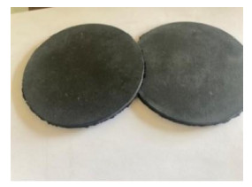
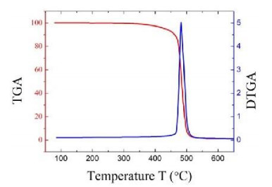
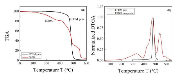
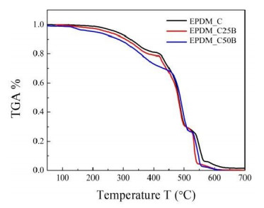
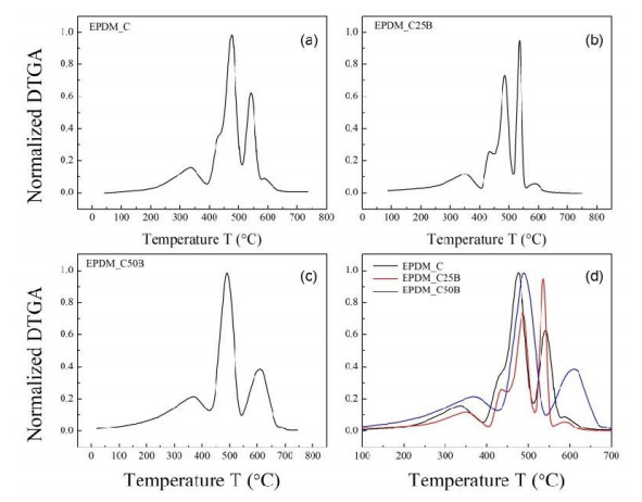
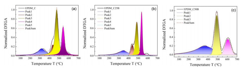
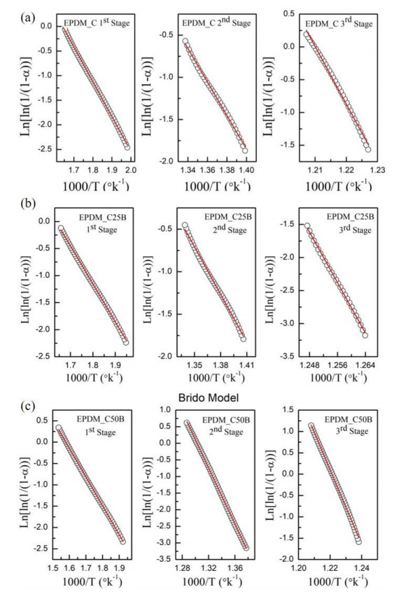
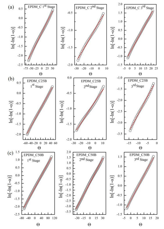
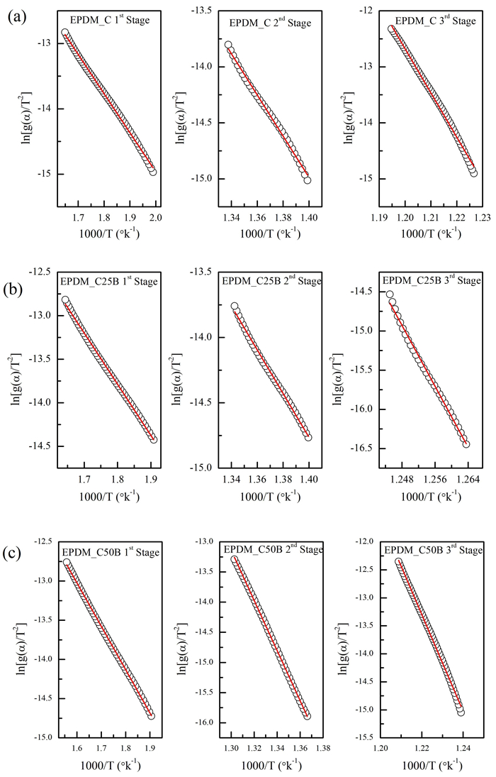
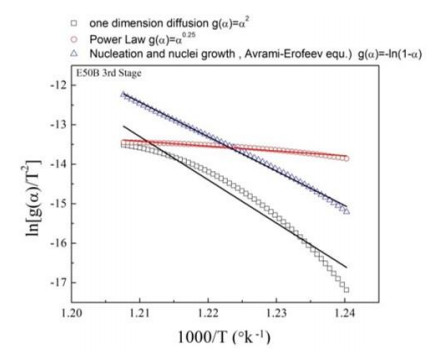
This research studies the effect of borax on the thermal stability and thermal kinetic behavior of ethylene-propylene-diene (EPDM) rubber composites. Using a laboratory two-roll mill at room temperature, carbon-black (N-220) as filler, and other additives such as zinc oxide, stearic acid, and paraffin oil were incorporated into the EPDM rubber matrix. The composite was prepared at different borax concentrations (25 and 50 phr). Thermogravimetric analysis was performed to characterize borax's effect onthermal stability before and after borax addition. Added borax to the host composite rubber (EPDM composite without borax) significantly improved the composite's thermal stability. Borax-loaded composites behave differently at various temperatures. To investigate the kinetic-thermal analysis of the prepared samples, three different models were applied. The activation energy (Ea) and frequency factors (A) for the Horowitz-Metzger, Broido and Coats-Redfern models were calculated. These models were compared and discussed based on their results. First-order decomposition also represented the main decomposition stage. Kraus and Cunnen-Russel models were used to test the interaction between rubber and borax based on previously published swelling results. No interaction was found between rubber and borax.
Citation: Alaa Ebrahiem, Sobhy S Ibrahim, Ahmed M El-Khaib, Ahmed S Doma. Ethylene-propylene-diene (EPDM) rubber/borax composite: kinetic thermal studies[J]. AIMS Materials Science, 2023, 10(4): 556-574. doi: 10.3934/matersci.2023031
This research studies the effect of borax on the thermal stability and thermal kinetic behavior of ethylene-propylene-diene (EPDM) rubber composites. Using a laboratory two-roll mill at room temperature, carbon-black (N-220) as filler, and other additives such as zinc oxide, stearic acid, and paraffin oil were incorporated into the EPDM rubber matrix. The composite was prepared at different borax concentrations (25 and 50 phr). Thermogravimetric analysis was performed to characterize borax's effect onthermal stability before and after borax addition. Added borax to the host composite rubber (EPDM composite without borax) significantly improved the composite's thermal stability. Borax-loaded composites behave differently at various temperatures. To investigate the kinetic-thermal analysis of the prepared samples, three different models were applied. The activation energy (Ea) and frequency factors (A) for the Horowitz-Metzger, Broido and Coats-Redfern models were calculated. These models were compared and discussed based on their results. First-order decomposition also represented the main decomposition stage. Kraus and Cunnen-Russel models were used to test the interaction between rubber and borax based on previously published swelling results. No interaction was found between rubber and borax.

| [1] |
Farajpour T, Bayat Y, Abdollahi M, et al. (2015) Effect of borax on the thermal and mechanical properties of ethylene‐propylene‐diene terpolymer rubber‐based heat insulator. J Appl Polym Sci 132: 41936. https://doi.org/10.1002/app.41936 doi: 10.1002/app.41936

|
| [2] |
Cavdar AD, Mengeloğlu F, Karakus K (2015) Effect of boric acid and borax on mechanical, fire and thermal properties of wood flour filled high density polyethylene composites. Measurement 60: 6–12. https://doi.org/10.1016/j.measurement.2014.09.078 doi: 10.1016/j.measurement.2014.09.078
|
| [3] | Kumar R, Gunjal J, Chauhan S (2022) Effect of borax-boric acid and ammonium polyphosphate on flame retardancy of natural fiber polyethylene composites. Maderas Cienc Tecnol 24. http://dx.doi.org/10.4067/s0718-221x2022000100434 |
| [4] | Dolotina CDC, Bo-ot LMT (2022) Effect of borax and boric acid on thermal and flammability properties of rice husk reinforced recycled HDPE composite. Athens J Technol Eng 9: 43–60. |
| [5] |
Wang J, Cao M, Li J, et al. (2022) Borate-modified, flame-retardant paper packaging materials for archive conservation. J Renew Mater 10: 1125–1136. http://dx.doi.org/10.32604/jrm.2022.018147 doi: 10.32604/jrm.2022.018147
|
| [6] |
Orhan R, Aydoğmuş E, Topuz S, et al. (2021) Investigation of thermo-mechanical characteristics of borax reinforced polyester composites. J Build Eng 42: 103051. https://doi.org/10.1016/j.jobe.2021.103051 doi: 10.1016/j.jobe.2021.103051
|
| [7] |
Abdulrahman ST, Ahmad Z, Thomas S, et al. (2020) Viscoelastic and thermal properties of natural rubber low‐density polyethylene composites with boric acid and borax. J Appl Polym Sci 137: 49372. https://doi.org/10.1002/app.49372 doi: 10.1002/app.49372
|
| [8] |
Habeeb SA, Hasan AS, Ţălu Ş, et al. (2021) Enhancing the properties of styrene-butadiene rubber by adding borax particles of different sizes. Iran J Chem Chem Eng 40: 1616–1629. https://doi.org/10.30492/ijcce.2020.40535 doi: 10.30492/ijcce.2020.40535
|
| [9] |
Takeno H, Inoguchi H, Hsieh WC (2020) Mechanical and structural properties of cellulose nanofiber/poly(vinyl alcohol) hydrogels cross-linked by a freezing/thawing method and borax. Cellulose 27: 4373–4387. https://doi.org/10.1007/s10570-020-03083-z doi: 10.1007/s10570-020-03083-z
|
| [10] |
More CV, Alsayed Z, Badawi MS, et al. (2021) Polymeric composite materials for radiation shielding: a review. Environ Chem Lett 19: 2057–2090. https://doi.org/10.1007/s10311-021-01189-9 doi: 10.1007/s10311-021-01189-9
|
| [11] |
Xu XR, Wu JQ, Xu J, et al. (2022) Preparation of flexible rubber composites with high contents of tungsten powders for gamma radiation shielding. Rare Metals 41: 2243–2248. https://doi.org/10.1007/s12598-021-01958-z doi: 10.1007/s12598-021-01958-z
|
| [12] |
Sayyed MI, Al-Ghamdi H, Almuqrin AH, et al. (2022) A study on the gamma radiation protection effectiveness of nano/micro-MgO-reinforced novel silicon rubber for medical applications. Polymers 14: 2867. https://doi.org/10.3390/polym14142867 doi: 10.3390/polym14142867
|
| [13] |
Abdulrahman ST, Patanair B, Vasukuttan VP, et al. (2022) High-density polyethylene/EPDM rubber blend composites of boron compounds for neutron shielding application. Express Polym Lett 16: 558–572. https://doi.org/10.3144/expresspolymlett.2022.42 doi: 10.3144/expresspolymlett.2022.42
|
| [14] |
Özdemir T, Yılmaz SN (2018) Mixed radiation shielding via 3-layered polydimethylsiloxane rubber composite containing hexagonal boron nitride, boron (Ⅲ) oxide, bismuth (Ⅲ) oxide for each layer. Radiat Phys Chem 152: 17–22. https://doi.org/10.1016/j.radphyschem.2018.07.007 doi: 10.1016/j.radphyschem.2018.07.007
|
| [15] |
Özdemir T, Yılmaz SN (2018) Hexagonal boron nitride and polydimethylsiloxane: a ceramic rubber composite material for neutron shielding. Radiat Phys Chem 152: 93–99. https://doi.org/10.1016/j.radphyschem.2018.08.008 doi: 10.1016/j.radphyschem.2018.08.008
|
| [16] |
Gamlin C, Markovic MG, Dutta NK, et al. (2000) Structural effects on the decomposition kinetics of EPDM elastomers by high-resolution TGA and modulated TGA. J Therm Anal Calorim 59: 319–336. https://doi.org/10.1023/A:1010164702571 doi: 10.1023/A:1010164702571
|
| [17] |
Alamgir M, Ghauri FA, Khan WQ, et al. (2021) Study of thermal behaviour of EPDM/SBR blends and carbon nanocoatings deposited by sputtering. Key Eng Mater 875: 116–120. https://doi.org/10.4028/www.scientific.net/KEM.875.116 doi: 10.4028/www.scientific.net/KEM.875.116
|
| [18] |
El-Nemr KF, Hassan MM, Masoaud EM, et al. (2021) Ablation and thermal properties of ethylene propylene diene rubber/carbon fiber composites cured by ionizing radiation for heat shielding applications. Egypt J Chem 64: 1471–1479. https://doi.org/10.21608/EJCHEM.2020.46989.2955 doi: 10.21608/EJCHEM.2020.46989.2955
|
| [19] |
Kissinger HE (1957) Reaction kinetics in differential thermal analysis. Anal Chem 29: 1702–1706. https://doi.org/10.1021/ac60131a045 doi: 10.1021/ac60131a045
|
| [20] | Friedman HL (1964) Kinetics of thermal degradation of char‐forming plastics from thermogravimetry. Application to a phenolic plastic. J Polym Sci Pol Sym 6: 183–195. https://doi.org/10.1002/polc.5070060121 |
| [21] |
Ozawa T (1965) A new method of analyzing thermogravimetric data. B Chem Soc Jpn 38: 1881–1886. https://doi.org/10.1246/bcsj.38.1881 doi: 10.1246/bcsj.38.1881
|
| [22] |
Ozawa T (1970) Kinetic analysis of derivative curves in thermal analysis. J Therm Anal 2: 301–324. https://doi.org/10.1007/BF01911411 doi: 10.1007/BF01911411
|
| [23] |
Horowitz HH, Metzger G (1963) A new analysis of thermogravimetric traces. Anal Chem 35: 1464–1468. https://doi.org/10.1021/ac60203a013 doi: 10.1021/ac60203a013
|
| [24] |
Sahoo A, Kumar S, Mohanty KA (2022) A comprehensive characterization of non-edible lignocellulosic biomass to elucidate their biofuel production potential. Biomass Convers Bior 12: 5087–5013. https://doi.org/10.1007/s13399-020-00924-6 doi: 10.1007/s13399-020-00924-6
|
| [25] | Ebrahiem A, El-Khatib AM, Doma AS (2023) Effect of lead and borax powder on the swelling behavior of EPDM rubber composite in toluene. Egypt J Chem. https://doi.org/10.21608/ejchem.2023.171647.7133 |
| [26] |
Ginic-Markovic M, Choudhury NR, Dimopoulos M, et al. (1998) Characterization of elastomer compounds by thermal analysis. Thermochim Acta 316: 87–95. https://doi.org/10.1016/S0040-6031(98)00290-1 doi: 10.1016/S0040-6031(98)00290-1
|
| [27] |
Wu K, Wang X, Xu Y, et al. (2020) Flame retardant efficiency of modified para-aramid fiber synergizing with ammonium polyphosphate on PP/EPDM. Polym Degrad Stabil 172: 109065. https://doi.org/10.1016/j.polymdegradstab.2019.109065 doi: 10.1016/j.polymdegradstab.2019.109065
|
Figures(10) / Tables(5)

Alaa Ebrahiem, Sobhy S Ibrahim, Ahmed M El-Khaib, Ahmed S Doma. Ethylene-propylene-diene (EPDM) rubber/borax composite: kinetic thermal studies[J]. AIMS Materials Science, 2023, 10(4): 556-574. doi: 10.3934/matersci.2023031


 DownLoad: