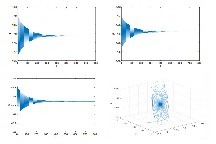
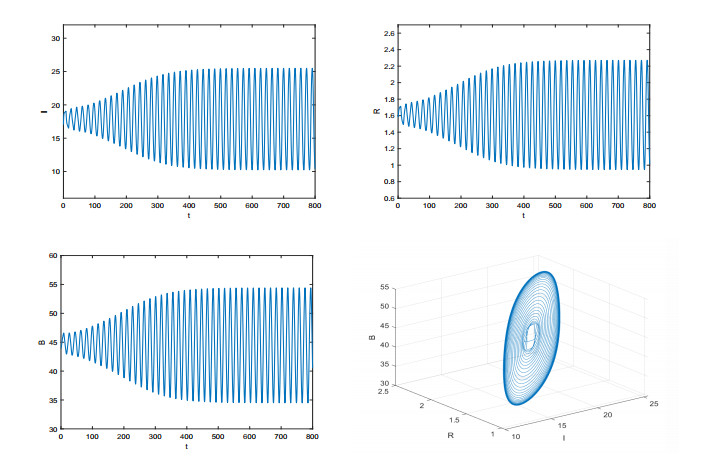
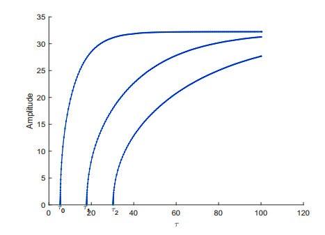
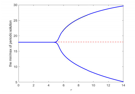
We propose a model for cholera under the impact of delayed mass media, including human-to-human and environment-to-human transmission routes. First, we establish the extinction and uniform persistence of the disease with respect to the basic reproduction number. Then, we conduct a local and global Hopf bifurcation analysis by treating the delay as a bifurcation parameter. Finally, we carry out numerical simulations to demonstrate theoretical results. The impact of the media with the time delay is found to not influence the threshold dynamics of the model, but is a factor that induces periodic oscillations of the disease.
Citation: Jie He, Zhenguo Bai. Global Hopf bifurcation of a cholera model with media coverage[J]. Mathematical Biosciences and Engineering, 2023, 20(10): 18468-18490. doi: 10.3934/mbe.2023820
We propose a model for cholera under the impact of delayed mass media, including human-to-human and environment-to-human transmission routes. First, we establish the extinction and uniform persistence of the disease with respect to the basic reproduction number. Then, we conduct a local and global Hopf bifurcation analysis by treating the delay as a bifurcation parameter. Finally, we carry out numerical simulations to demonstrate theoretical results. The impact of the media with the time delay is found to not influence the threshold dynamics of the model, but is a factor that induces periodic oscillations of the disease.

| [1] |
N. Wang, L. Qi, M. Bessane, M. Hao, Global Hopf bifurcation of a two-delay epidemic model with media coverage and asymptomatic infection, J. Differ. Equations, 369 (2023), 1–40. https://doi.org/10.1016/j.jde.2023.05.036 doi: 10.1016/j.jde.2023.05.036

|
| [2] |
Y. Xiao, S. Tang, J. Wu, Media impact switching surface during an infectious disease outbreak, Sci. Rep., 5 (2015), 7838. http://doi.org/10.1038/srep07838 doi: 10.1038/srep07838
|
| [3] |
J. Cui, Y. Sun, H. Zhu, The impact of media on the control of infectious diseases, J. Dyn. Differ. Equations, 20 (2008), 31–53. http://doi.org/10.1007/s10884-007-9075-0 doi: 10.1007/s10884-007-9075-0
|
| [4] |
Y. Li, J. Cui, The effect of constant and pulse vaccination on SIS epidemic models incorporating media coverage, Commun. Nonlinear Sci. Numer. Simul., 14 (2009), 2353–2365. https://doi.org/10.1016/j.cnsns.2008.06.024 doi: 10.1016/j.cnsns.2008.06.024
|
| [5] |
R. Liu, J. Wu, H. Zhu, Media/psychological impact on multiple outbreaks of emerging infectious diseases, Comput. Math. Methods Med., 8 (2007), 153–164. http://doi.org/10.1080/17486700701425870 doi: 10.1080/17486700701425870
|
| [6] |
Y. Xiao, T. Zhao, S. Tang, Dynamics of an infectious diseases with media/psychology induced non-smooth incidence, Math. Biosci. Eng., 10 (2013), 445–461. https://doi.org/10.3934/mbe.2013.10.445 doi: 10.3934/mbe.2013.10.445
|
| [7] |
S. Collinson, J. Heffernan, Modeling the effects of media during an influenza epidemic, BMC Public Health, 14 (2014), 376. https://doi.org/10.1186/1471-2458-14-376 doi: 10.1186/1471-2458-14-376
|
| [8] |
Q. Yan, S. Tang, J. Wu, S. Gabriele, Media coverage and hospital notifications: correlation analysis and optimal media impact duration to manage a pandemic, J. Theor. Biol., 390 (2016), 1–13. https://doi.org/10.1016/j.jtbi.2015.11.002 doi: 10.1016/j.jtbi.2015.11.002
|
| [9] |
C. Yang, J. Wang, A cholera transmission model incorporating the impact of medical resources, Math. Biosci. Eng., 16 (2019), 5226–5246. https://doi.org/10.3934/mbe.2019261 doi: 10.3934/mbe.2019261
|
| [10] |
P. Song, Y. Xiao, Global hopf bifurcation of a delayed equation describing the lag effect of media impact on the spread of infectious disease, J. Math. Biol., 76 (2018), 1249–1267. https://doi.org/10.1007/s00285-017-1173-y doi: 10.1007/s00285-017-1173-y
|
| [11] |
T. Zhao, M. Zhao, Global hopf bifurcation analysis of an susceptible-infective-removed epidemic model incorporating media coverage with time delay, J. Biol. Dyn., 11 (2017), 8–24. https://doi.org/10.1080/17513758.2016.1229050 doi: 10.1080/17513758.2016.1229050
|
| [12] |
Z. Mukandavire, S. Liao, J. Wang, H. Gaff, D. L. Smith, J. G. Morris, Estimating the reproductive numbers for the 2008–2009 cholera outbreaks in Zimbabwe, Proc. Natl. Acad. Sci. USA, 108 (2011), 8767–8772. https://doi.org/10.1073/pnas.1019712108 doi: 10.1073/pnas.1019712108
|
| [13] |
J. Wang, X. Wang, D. Gao, Influence of human behavior on cholera dynamics, Math. Biosci., 267 (2015), 41–52. https://doi.org/10.1016/j.mbs.2015.06.009 doi: 10.1016/j.mbs.2015.06.009
|
| [14] |
L. Zhang, Z. Wang, Y. Zhang, Dynamics of a reaction-diffusion waterborne pathogen model with direct and indirect transmission, Comput. Math. Appl., 72 (2016), 202–215. https://doi.org/10.1016/j.camwa.2016.04.046 doi: 10.1016/j.camwa.2016.04.046
|
| [15] |
G. Sun, J. Xie, S. Huang, Z. Jin, M. Li, L. Liu, Transmission dynamics of cholera: mathematical modeling and control strategies, Commun. Nonlinear Sci. Numer. Simul., 45 (2017), 235–244. https://doi.org/10.1016/j.cnsns.2016.10.007 doi: 10.1016/j.cnsns.2016.10.007
|
| [16] |
J. Wang, J. Wang, Analysis of a reaction-diffusion cholera model with distinct dispersal rates in the human population, J. Dyn. Differ. Equations, 33 (2021), 549–575. http://doi.org/10.1007/s10884-019-09820-8 doi: 10.1007/s10884-019-09820-8
|
| [17] |
H. Shu, Z. Ma, X. Wang, Threshold dynamics of a nonlocal and delayed cholera model in a spatially heterogeneous environment, J. Math. Biol., 83 (2021), 41. https://doi.org/10.1007/s00285-021-01672-5 doi: 10.1007/s00285-021-01672-5
|
| [18] |
J. Wang, Mathematical models for cholera dynamics-a review, Microorganisms, 10 (2022), 2358. https://doi.org/10.3390/microorganisms10122358 doi: 10.3390/microorganisms10122358
|
| [19] | J. Hale, S. Lunel, Introduction to Functional Differential Equations, Springer, New York, 1993. Available from: https://link.springer.com/book/10.1007/978-1-4612-4342-7. |
| [20] | H. Smith, Monotone Dynamical Systems: An Introduction to the Theory of Competitive and Cooperative Systems, American Mathematical Society, Providence, RI, 1995. https://doi.org/10.1090/surv/041 |
| [21] |
P. Driessche, J. Watmough, Reproduction numbers and sub-threshold endemic equilibria for compartmental models of disease transmission, Math. Biosci., 180 (2002), 29–48. https://doi.org/10.1016/S0025-5564(02)00108-6 doi: 10.1016/S0025-5564(02)00108-6
|
| [22] |
J. Hale, Dynamical systems and stability, J. Math. Anal. Appl., 26 (1969), 39–59. https://doi.org/10.1016/0022-247X(69)90175-9 doi: 10.1016/0022-247X(69)90175-9
|
| [23] | J. Hale, Asymptotic Behavior of Dissipative Systems, American Mathematical Society, Providence, 25 (1988). https://doi.org/10.1090/surv/025 |
| [24] | X. Zhao, Dynamical Systems in Population Biology, 2nd edition, Springer, New York, 2017. https://doi.org/10.1007/978-3-319-56433-3 |
| [25] | X. Zhao, Uniform persistence and periodic coexistence states in infinite-dimensional periodic semiflows with applications, Can. Appl. Math. Q., 3 (1995), 473–495. Available from: https://www.math.mun.ca/~zhao/Selectpapers/Zhao1995CAMQpub.pdf. |
| [26] |
R. Corless, G. Gonnet, D. Hare, D. Jeffrey, D. Knuth, On the LambertW function, Adv. Comput. Math., 5 (1996), 329–359. https://doi.org/10.1007/BF02124750 doi: 10.1007/BF02124750
|
| [27] |
M. Y. Li, J. Muldoweny, A geometric approach to the global-stability problems, SIAM J. Math. Anal., 27 (1996), 1070–1083. https://doi.org/10.1137/S0036141094266449 doi: 10.1137/S0036141094266449
|
| [28] | J. Muldowney, Compound matrices and ordinary differential equations, Rocky. Mt. J. Math., 20 (1990), 857–872. Available from: https://www.jstor.org/stable/44237627. |
| [29] | W. Coppel, Stability and Asymptotic Behavior of Differential Equations, Health, Boston, 1995. |
| [30] |
P. Song, Y. Xiao, Analysis of an epidemic system with two response delays in media impact function, Bull. Math. Biol., 81 (2019), 1582–1612. https://doi.org/10.1007/s11538-019-00586-0 doi: 10.1007/s11538-019-00586-0
|
| [31] |
J. Wu, Symmetric functional differential equations and neural networks with memory, Trans. Am. Math. Soc., 350 (1998), 4799–4838. https://doi.org/10.1090/S0002-9947-98-02083-2 doi: 10.1090/S0002-9947-98-02083-2
|
| [32] |
J. Wei, M. Y. Li, Hopf bifurcation analysis in a delayed Nicholson blowflies equation, Nonlinear Anal., 60 (2005), 1351–1367. https://doi.org/10.1016/j.na.2003.04.002 doi: 10.1016/j.na.2003.04.002
|
| [33] |
H. Shu, L. Wang, J. Wu, Global dynamics of Nicholson's blowflies equation revisited: onset and termination of nonlinear oscillations, J. Differ. Equations, 255 (2013), 2565–2586. https://doi.org/10.1016/j.jde.2013.06.020 doi: 10.1016/j.jde.2013.06.020
|
| [34] |
H. Shu, G. Fan, H. Zhu, Global hopf bifurcation and dynamics of a stage–structured model with delays for tick population, J. Differ. Equations, 284 (2021), 1–22. https://doi.org/10.1016/j.jde.2021.02.037 doi: 10.1016/j.jde.2021.02.037
|
| [35] |
X. Zhang, F. Scarabel, X. Wang, J. Wu, Global continuation of periodic oscillations to a diapause rhythm, J. Dyn. Differ. Equations, 34 (2022), 2819–2839. https://doi.org/10.1007/s10884-020-09856-1 doi: 10.1007/s10884-020-09856-1
|
| [36] | J. Wei, H. Wang, W. Jiang, Bifurcation Theory of Delay Differential Equations, Science Press, 2012. |
| [37] | K. Engelborghs, T. Luzyanina, G. Samaey, DDE-BIFTOOL v. 2.00: A Matlab package for bifurcation analysis of delay differential equations, Technical Report TW-330, KU Leuven, Belgium, 2001. Available from: https://www.researchgate.net/publication/245840825. |
| [38] |
K. Engelborghs, T. Luzyanina, D. Roose, Numerical bifurcation analysis of delay differential equations using DDE-BIFTOOL, ACM Trans. Math. Software, 28 (2002), 1–21. https://doi.org/10.1145/513001.513002 doi: 10.1145/513001.513002
|
| [39] |
H. Shu, X. Hu, L. Wang, J. Watmough, Delay induced stability switch, multitype bistability and chaos in an intraguild predation model, J. Math. Biol., 71 (2015), 1269–1298. https://doi.org/10.1007/s00285-015-0857-4 doi: 10.1007/s00285-015-0857-4
|
Figures(4)

Jie He, Zhenguo Bai. Global Hopf bifurcation of a cholera model with media coverage[J]. Mathematical Biosciences and Engineering, 2023, 20(10): 18468-18490. doi: 10.3934/mbe.2023820


 DownLoad: