


Infectious diseases have been one of the major causes of human mortality, and mathematical models have been playing significant roles in understanding the spread mechanism and controlling contagious diseases. In this paper, we propose a delayed SEIR epidemic model with intervention strategies and recovery under the low availability of resources. Non-delayed and delayed models both possess two equilibria: the disease-free equilibrium and the endemic equilibrium. When the basic reproduction number R0=1, the non-delayed system undergoes a transcritical bifurcation. For the delayed system, we incorporate two important time delays: τ1 represents the latent period of the intervention strategies, and τ2 represents the period for curing the infected individuals. Time delays change the system dynamics via Hopf-bifurcation and oscillations. The direction and stability of delay induced Hopf-bifurcation are established using normal form theory and center manifold theorem. Furthermore, we rigorously prove that local Hopf bifurcation implies global Hopf bifurcation. Stability switching curves and crossing directions are analyzed on the two delay parameter plane, which allows both delays varying simultaneously. Numerical results demonstrate that by increasing the intervention strength, the infection level decays; by increasing the limitation of treatment, the infection level increases. Our quantitative observations can be useful for exploring the relative importance of intervention and medical resources. As a timing application, we parameterize the model for COVID-19 in Spain and Italy. With strict intervention policies, the infection numbers would have been greatly reduced in the early phase of COVID-19 in Spain and Italy. We also show that reducing the time delays in intervention and recovery would have decreased the total number of cases in the early phase of COVID-19 in Spain and Italy. Our work highlights the necessity to consider the time delays in intervention and recovery in an epidemic model.
Citation: Sarita Bugalia, Jai Prakash Tripathi, Hao Wang. Mathematical modeling of intervention and low medical resource availability with delays: Applications to COVID-19 outbreaks in Spain and Italy[J]. Mathematical Biosciences and Engineering, 2021, 18(5): 5865-5920. doi: 10.3934/mbe.2021295
| [1] | Guilherme Giovanini, Alan U. Sabino, Luciana R. C. Barros, Alexandre F. Ramos . A comparative analysis of noise properties of stochastic binary models for a self-repressing and for an externally regulating gene. Mathematical Biosciences and Engineering, 2020, 17(5): 5477-5503. doi: 10.3934/mbe.2020295 |
| [2] | Zhenquan Zhang, Junhao Liang, Zihao Wang, Jiajun Zhang, Tianshou Zhou . Modeling stochastic gene expression: From Markov to non-Markov models. Mathematical Biosciences and Engineering, 2020, 17(5): 5304-5325. doi: 10.3934/mbe.2020287 |
| [3] | Qiuying Li, Lifang Huang, Jianshe Yu . Modulation of first-passage time for bursty gene expression via random signals. Mathematical Biosciences and Engineering, 2017, 14(5&6): 1261-1277. doi: 10.3934/mbe.2017065 |
| [4] | Heli Tan, Tuoqi Liu, Tianshou Zhou . Exploring the role of eRNA in regulating gene expression. Mathematical Biosciences and Engineering, 2022, 19(2): 2095-2119. doi: 10.3934/mbe.2022098 |
| [5] | Jiajun Zhang, Tianshou Zhou . Stationary moments, distribution conjugation and phenotypic regions in stochastic gene transcription. Mathematical Biosciences and Engineering, 2019, 16(5): 6134-6166. doi: 10.3934/mbe.2019307 |
| [6] | Qi Wang, Lifang Huang, Kunwen Wen, Jianshe Yu . The mean and noise of stochastic gene transcription with cell division. Mathematical Biosciences and Engineering, 2018, 15(5): 1255-1270. doi: 10.3934/mbe.2018058 |
| [7] | Pierre Degond, Maxime Herda, Sepideh Mirrahimi . A Fokker-Planck approach to the study of robustness in gene expression. Mathematical Biosciences and Engineering, 2020, 17(6): 6459-6486. doi: 10.3934/mbe.2020338 |
| [8] | Xuan Zhang, Huiqin Jin, Zhuoqin Yang, Jinzhi Lei . Effects of elongation delay in transcription dynamics. Mathematical Biosciences and Engineering, 2014, 11(6): 1431-1448. doi: 10.3934/mbe.2014.11.1431 |
| [9] | Gerardo Aquino, Andrea Rocco . Bimodality in gene expression without feedback: from Gaussian white noise to log-normal coloured noise. Mathematical Biosciences and Engineering, 2020, 17(6): 6993-7017. doi: 10.3934/mbe.2020361 |
| [10] | Qiqi Deng, Aimin Chen, Huahai Qiu, Tianshou Zhou . Analysis of a non-Markov transcription model with nuclear RNA export and RNA nuclear retention. Mathematical Biosciences and Engineering, 2022, 19(8): 8426-8451. doi: 10.3934/mbe.2022392 |
Infectious diseases have been one of the major causes of human mortality, and mathematical models have been playing significant roles in understanding the spread mechanism and controlling contagious diseases. In this paper, we propose a delayed SEIR epidemic model with intervention strategies and recovery under the low availability of resources. Non-delayed and delayed models both possess two equilibria: the disease-free equilibrium and the endemic equilibrium. When the basic reproduction number R0=1, the non-delayed system undergoes a transcritical bifurcation. For the delayed system, we incorporate two important time delays: τ1 represents the latent period of the intervention strategies, and τ2 represents the period for curing the infected individuals. Time delays change the system dynamics via Hopf-bifurcation and oscillations. The direction and stability of delay induced Hopf-bifurcation are established using normal form theory and center manifold theorem. Furthermore, we rigorously prove that local Hopf bifurcation implies global Hopf bifurcation. Stability switching curves and crossing directions are analyzed on the two delay parameter plane, which allows both delays varying simultaneously. Numerical results demonstrate that by increasing the intervention strength, the infection level decays; by increasing the limitation of treatment, the infection level increases. Our quantitative observations can be useful for exploring the relative importance of intervention and medical resources. As a timing application, we parameterize the model for COVID-19 in Spain and Italy. With strict intervention policies, the infection numbers would have been greatly reduced in the early phase of COVID-19 in Spain and Italy. We also show that reducing the time delays in intervention and recovery would have decreased the total number of cases in the early phase of COVID-19 in Spain and Italy. Our work highlights the necessity to consider the time delays in intervention and recovery in an epidemic model.
Abbreviations: BOD: Biochemical Oxygen Demand; COD: Chemical Oxygen Demand; WHO: World Health Organization; BOD5: 5-day Biochemical Oxygen Demand; ECA: Environment Conservation Amendment; DO: Demand for Oxygen; DWASA: Dhaka Water Supply & Sewerage Authority; TSS: Toxic Shock Syndrome; AS: Surface Area; N: Nitrogen; P: Phosphorus; EPA: Environmental Protection Agency; KWASA: Khulna Water Supply & Sewerage Authority; LGED: Local Govt. Engineering Department; TN: Tri-nitro Toluene
Municipal wastewater is the conveyed wastes from homes, business offices or modern industries, notwithstanding any groundwater, surface water, and tempest water that might be available. Untreated wastewater, for the most part, contains elevated amounts of natural material, various pathogenic micro-organisms, and in addition supplements and dangerous mixes. It along these lines involves ecological dangers and thus should promptly be passed on far from its sources and treated properly before definite transfer. An objective of wastewater treatment is the security of the earth water, they say is life, to say the truth they are correct. But the accessibility of water is becoming a great concern nowadays in the globalized world, both in developing and developed countries. A sustainable employ of water sources could result in the search of supplementary water sources or even in recycling wastewater treatment plant effluents [1,2]. Waste water treatment is a process which is used to turn waste water into an effluent, that can be returned to the water cycle with no or minimal impact to the environment. This treated waste water can be used for many other purposes. Figure 1 shows a typical configuration of waste water treatment process. Wastewater from home must be treated in an environmentally friendly manner so that it can be reused. In the system, screening is considered as the very first process where wastewater is cleaned (removal of course particles i.e. cotton buds, sanitary items, face wipes, glass particles and etc.); in this process, no heavy machinery is employed. After this, the primary treatment is applied, where organic/solid materials are separated from the water. It is generally done by putting the screened water into settlement tanks so that the solids can sink at the bottom of the tank. The rest of the process is termed secondary treatment; high removal of BOD, COD and toxic materials are ensured at this stage. Primary treated water is stored in rectangular shaped tanks (Aeration Lane) and the air is pumped inside to meet the DO. Lastly, sludge is all over again cleaned and scrapped by sand filter bed resulting in edible water to be reused.
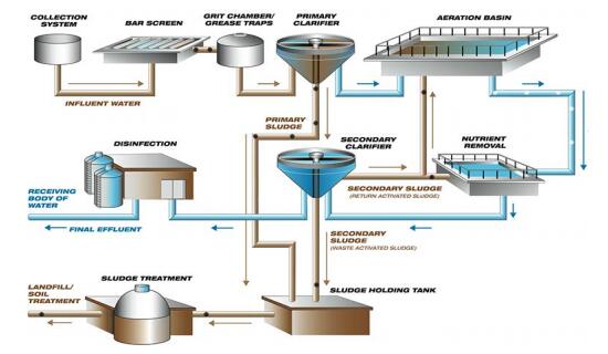 Figure 1. Typical waste water treatment process.
Bangladesh is a developing country, where water treatment and sanitation are currently facing tremendous challenges. Bangladesh has developed in water accessibility and arsenic reduction from various sources of water even though having various internal problems. Responsiveness about sanitation and hygiene has been enhanced considerably in recent times. A number of local and international organizations are trying to lessen the water-related issues. Many initiatives have been taken to set up tube wells for safe water sources. But the quality of water from those tube wells is now and then contaminated. Around 11% of death by diarrhea is associated with the use of unprocessed groundwater [3]. Pollution is more severe in areas with clay and slit layers. In accumulation, indecent placement of latrines and discharge of unprocessed effluent in the surface water are creating more severe infectivity.
In Bangladesh, underground water layer diminution is one of the most significant issues. A research of 2011 shows that in Bangladesh, diminution of groundwater was around 0.01–0.05 m/year. Over the last 50 years, the growth of extraction of groundwater was 20–260 km3/year [4]. Water extraction for cultivation by deep tube wells are the main sector of groundwater pollution. The condition of water infectivity is quite different in urban and rural areas. Water scarcity is a serious issue in urban areas; as on-ground water is infected by toxic effluent discharge. In rural areas, relatively more people have user-friendliness to water sources. In the past few years, arsenic was a major issue for the people of Bangladesh. Somehow, this condition is overcome by making significant efforts to decrease this problem. Rural areas still lag in treatment conveniences of wastewater. Village residents discharge wastewater is almost untreated to the nearest water bodies, though there is an enormous potential of this wastewater to be reused in agricultural fields. Such initiative will not only reduce groundwater demand but can also serve as a healthier environment if accurate treatment is provided.
Several works have been done on waste water treatment in the last few years. Deborah Panepinto et al. anticipated a research presents a multi-step methodology for the assessment of the energetic aspects of wastewater treatment, which was implemented on the largest city in Italy (2.7 M population equivalents as organic load), managed by Società Metropolitana Acque Torino (SMAT) [5]. Waste water treatment high rate algal ponds (WWT HRAPs) are a gifted technology that could help to solve water pollution challenges concomitantly where climate condition is favorable. Generally, 800–1400 GJ/ha/year energy (average biomass energy content: 20 GJ/ton; HRAP biomass productivity: 40–70 tons/ha/year) can be generated in the form of harvestable biomass from WWT HRAP, which eventually can be used to fulfill community-level energy demand [6]. Chen et al. showed different electrochemical techniques for treating wastewater. Though all the systems were effective all of them had very high initial cost and there was a huge chance of chemical exposure [7]. Crini et al. reviewed 4 types of the treatment system and researched on the absorbent based biological treatment process. The system was only applicable for industries and high scale treatment process; cost is moderate but high risk of contamination via absorbents [8]. Liu et al. worked on three types of chemical system to purify industrial wastewater and did a development plant to produce electricity in the meantime of purification by using a single microbial fuel cell. The researchers mainly focused to produce electricity and systems had the low effectiveness of treatment process [9]. Le-Clech et al. did a research on membrane utilized treatment system via bio-reactor; used osmosis and reverse osmosis process to treat wastewater. Bio-reactors are very tough to settle and only applicable for the non-tropical region [10]. Kampschreur et al. conducted a research project on water treatment plants and determined the adverse effects of different centralized treatment processes. The system was effective but a huge amount of NOx was produced while implementing [11]. Singh et al. did a compact review on treating water using microbial fuel cells along with electricity generation, showed various drawbacks of this process. It has higher efficiency, but it hampers the normal living of micro-organisms of the pond [12]. Fu et al. reviewed various treatment process and found zero-valence iron to be an effective treatment effluent. Only natural treatment processes can use zero-valence iron. High risk of iron ion contamination in groundwater was the major deficiency of the plant [13]. Yuan et al. did a research on urban areas on waste water treatment processes using a decentralized technique. This process is also applicable for urban areas where the underwater level is good enough [14]. Seto et al. did a case study on centralized treatment process on San Francisco and found that centralized systems the higher possibility of micro-organism contamination [15]. Ms. Ayesha Sharmin did a master thesis about introducing de-centralized treatment technology on Bangladesh on 2016 at Lund University where she described the pros and cons about that technology very clearly [16].
All the above electrochemical processes are very much costly and the other processes were invented for industrial and urban wastewater treatment and a large population. These plants are not very much effective while Bangladesh is a poor country and most of the people live under the poverty line. For Khulna district of Bangladesh, it is necessary to find or invent a method to treat water which would be efficient and can be implemented at low cost. In April, 2018, Avijit Mallik and Md. Arman Arefin published a research about introducing and design of a de-centralize treatment plant for southern Bangladesh [17]. This research is the extended part of the previous one. In this paper, a new technique is designed and discussed for decentralized wastewater treatment with primary and secondary treatment processes which has high efficiency and plant initial and running cost is low. This plant is very much effective for a big family or three-four small families. All the designed sections are discussed and their advantages and disadvantages are evaluated from the perspective of rural areas of Bangladesh. Detailed feasibility analysis of the designed plant is conducted including installation cost and payback period.
According to Bangladesh national drinking water survey 2009, "22 million people are still drinking water that does not meet the standard level for arsenic of 0.05 mg/L and 5.6 million are in high risk of having water with more than 0.2 mg/L arsenic" [18]. Table 1 shows the standard values of different elements in water according to Department of Public Health Engineering and World Health Organization. Some common elements have been selected in this table. In recent few years, arsenic was a very big issue of concern for Bangladesh. BOD, COD, nitrate, phosphate, and chloride are very important elements for drinking water. An excessive amount of these elements can cause a health hazard. Drinking water should contain the following elements according to the standard stated in Table 1 [19].
| Sl. No. | Water Quality Parameters |
Bangladesh Standards (mg/L) | WHO Guide Line |
Methods/Equipment |
| 01 | Aluminum | 0.2 | − | Atomic Absorption Apectro-photometer (AAS) |
| 02 | Ammonia | 0.5 | UV-VIS | |
| 03 | Arsenic | 0.05 | 0.01 | AAS |
| 04 | Barium | 0.01 | 0.7 | AAS |
| 05 | Benzene | 0.01 | 0.01 | Gas Chromatograph |
| 06 | BOD 5 day, 20 ℃ | 0.2 | − | 5 days Incubation |
| 07 | Boron | 1.0 | − | UV-VIS |
| 08 | Cadmium | 0.005 | 0.003 | AAS |
| 09 | Calcium | 75 | − | AAS |
| 10 | Chloride | 150–600 | − | Titrimetric |
| 11 | Chlorinated Alkenes | |||
| 11.1 | Carbontetrachloride | 0.01 | 0.004 | Gas Chromatograph |
| 11.2 | 1.1 DichloroEthelene | 0.001 | 0.03 | Gas Chromatograph |
| 11.3 | 1.2 DichloroEthelene | 0.03 | 0.03 | Gas Chromatograph |
| 11.4 | TetrachloroEthelene | 0.03 | 0.04 | Gas Chromatograph |
| 11.5 | TrichloroEthelene | 0.09 | 0.07 | Gas Chromatograph |
| 12.1 | Pentachlorophenol | 0.03 | 0.009 | Gas Chromatograph |
| 12.2 | 2, 4, 6-Trichlorophenol | 0.03 | 0.2 | Gas Chromatograph |
| 13 | Chlorine (Residual) | 0.2 | − | Titrimetric |
| 14 | Chloroform | 0.09 | 0.2 | Gas Chromatograph |
| 15 | Chromium (Hexavalent) | 0.05 | − | Iron Chromatograph |
| 16 | Chromium (Total) | 0.05 | 0.05 (P) | AAS |
| 17 | COD | 4 | − | Closed Reflux Method |
| 18 | Coli form (Fecal) | 0 CFU (N/100 mL) | 0 | Membrane Filtration Method |
| 19 | Coli form (Total) | 0 CFU (N/100 mL) | 0 | Membrane Filtration Method |
| 20 | Color | 15 Hazen | − | Color Comparator |
| 21 | Copper | 1 | 2 | AAS |
| 22 | Cyanide | 0.1 | 0.07 | UV-VIS/Specific Ion Electrode |
| 23 | Detergent | 0.2 | − | UV-VIS |
| 24 | DO | 6 | − | Multimeter |
| 25 | Electric Conductivity | −us/cm | − | Multimeter |
| 26 | Fluoride | 1 | 1.5 | UV-VIS |
| 27 | Hardness as CaCO3 | 200–500 | − | Titrimetric |
| 28 | Iodine | 200–500 | − | Titrimetric |
| 29 | Iron | 0.3–1.0 | − | AAS |
| 30 | Nitrogen (Total) | 1 | − | UV-VIS/Digestion |
| 31 | Lead | 0.05 | 0.01 | AAS |
| 32 | Magnesium | 30–35 | − | AAS |
| 33 | Manganese | 0.1 | − | AAS |
| 34 | Mercury | 0.001 | 0.001 | Mercury Analyzer |
| 35 | Nickel | 0.1 | 0.02 (P) | AAS |
| 36 | Nitrate | 10 | 50.0 as N | UV-VIS |
| 37 | Nitrite | < 1 | 3.0 (0.2) | UV-VIS |
| 38 | Odor | Odorless | − | Threshold Method |
| 39 | ORP (Eh) | − | − | ORP meter |
| 40 | Oil and Grease | 0.01 | − | Oil and Grease meter |
| 41 | pH | 6.5–8.5 | pH Meter | |
| 42 | Phenolic Compounds | 0.002 | − | Gas Chromatograph |
| 43 | Phosphate | 6 | − | UV-VIS |
| 44 | Phosphorus | 0 | − | Digestion |
| 45 | Potassium | 12 | − | AAS |
| 46 | Radioactive Materials (Gross Alpha Activity) | 0.01 Bq/L | 0.5 Bq/L | − |
| 47 | Radioactive Materials (Gross Beta Activity) | 0.1 Bq/L | 1.0 Bq/L | − |
| 48 | Salinity | − | − | Multimeter |
| 49 | Selenium | 0.01 | 0.01 | AAS |
| 50 | Silver | 0.02 | − | AAS |
| 51 | Sodium | 200 | − | AAS |
| 52 | Suspended Solids | 10 | − | Filtration and Drying |
| 53 | Sulphide | 0 | − | UV-VIS |
| 54 | Sulphate | 400 | − | UV-VIS |
| 55 | Taste | − | − | Threshold Method |
| 56 | Total Alkalinity | − | − | Titrimetric |
| 57 | Total Dissolved Solid | 1000 | − | Multimeter |
| 58 | Temperature | 20–30 C | Thermometer | |
| 59 | Tin | 2 | − | AAS |
| 60 | Turbidity | 10 NTU | − | Turbidity meter |
| 61 | Zinc | 5 | − | AAS |
 DownLoad: CSV
The survey also stated that "98% of the tested samples meet the Bangladesh standard of 600 mg/L for chloride concentration". Fluoride concentration was not so high according to this survey. Six samples (1%) exceeded the Bangladesh standard of 1.1–1.5 mg/L. But, iron concentration seems to be a little bit concerning in the edible water. Throughout the country, only 60% of the tested samples meet the national standard of 1 mg/L iron. The other 40% is below the standard. The amount of phosphorus in almost 93% of the sample meet the standard value 1.96 mg/L, which is equivalent to 6 mg/L phosphate.
In Dhaka city, normally water is pumped from deep aquifers. However, the quality does not remain similar to the consumers. Along with its transport through the pipe network, a number of sources cause contamination of the water. The negative pressure of the pump, leakage in the pipes, service installation networks under septic tanks etc. are reasons behind water contamination in the pipe network [20]. Bangladesh government has introduced rules and regulations to protect their water and environment. Different governmental organizations, as well as NGOs, work for implementing regulations. The Department of Environment (DoE) is a government organization, it works on that basis. This organization has created a mobile court in order to implement action against environment conservation violator under the ECA Act, 2010. "Polluters pay principal" is mentioned in the ECA, 1995 [21]. Table 2 represents guidelines for different parameters in surface water. Surface water used by different activity should maintain the concentration of various parameters according to the table below [18,19].
| Parameter | Irrigation | Agriculture | Drinking | Treated Values |
| pH | 6–8.73 | 6.00–8 | 6.5–8.5 | 6–6.5 |
| EC (Us/m) | 0–3.00 | 0.20–0.25 | 0.25 | 0.3–0.4 |
| DO (ppm) | 4.25–5 | 5 | 3.5–5 | 3–4.8 |
| TDS (ppm) | 0–1900 | 150 | 450–510 | 350–420 |
| Total Nitrogen (ppm) | 0–32.00 | 0–0.1 | 1 | 4–4.9 |
| Phosphorus (ppm) | 0–2 | 0–0.1 | N/A | 9.8–10 |
| Cadmium (ppm) | 0–0.0125 | 0.25–1.8 | 0–0.002 | 0 |
| Iron (ppm) | 3.5–5.00 | 0.2 | 0–0.068 | 1.5–1.75 |
| Manganese (ppm) | 0–0.22 | 0–0.009 | 0–0.02 | 0.15 |
DownLoad: CSVThe National Environment Management Action Plan (NEMAP), 1995 includes identification of major environmental issues and action to minimize environmental degradation improving natural environment by conserving biodiversity. The different international organization also helps financially by providing a fund for implementing environmental regulations in Bangladesh namely DANIDA, SIDA, USAID, CIDA etc. [22].
In urban areas, DWASA is responsible for treating potable water for the community, in the capital city Dhaka. DWASA is currently running one large and three small water treatment plants with financial assistance from different funding organizations. According to the department of public health and engineering of Bangladesh, most of the treatment facilities include filtration, flocculation, sedimentation, and disinfection. Some also include ion exchange and filtration depending on the quality of collected water. A groundwater rule is developing to specify the appropriate use of disinfection to assure public health protection.
However, to meet the fastest growing water demand and reduce groundwater extraction, DWASA planned to build four large surface water treatment plants until 2021. These plants have been proposed to draw water from less polluted surface water even though they are distant sources such as rivers. The four plants are expected to have a combined capacity of 1.63 million cubic meters surface water per day, whereas in 2010 the supply of groundwater was 2.11 million cubic meters per day [23,24].
Easy availability and no content of pathogenic microorganisms make groundwater so popular that most of the rural population is now dependent on low-cost tube wells. Studies stated that Bangladesh achieved a remarkable success providing 97% of the rural population with bacteriologically safe tube well water. In some regions where tube well's water is not trusted worthy, people usually boil water for purification. Arsenic contamination is one of the major challenges in the shallow aquifers and many parts of the country have made shallow tube well water unsafe for drinking. Different strategies have been developed to mitigate the arsenic problem. Those are classified as chemical and non-chemical treatment. Pond sand filters dug and ring well, chili water purifiers (CWP) are some nonchemical solution for arsenic contamination. Chulli water purifier is a special type of clay oven with the metal coil. Water is passing through the coil and gets purified from arsenic by heat. Chemical options include different types of filters such as SIDKO, SONO, READ F, and AIKAN [25].
The current research is mainly focused on wastewater treatment. In this paper, a new economical wastewater treatment process for the rural areas has been proposed and designed. The process is mainly a de-centralized water treatment technique. Decentralized wastewater treatment does not mean one specific plant for the whole population in a defined area but it rather defines more than one or an assortment of technologies. The system is mainly designed for a low to moderate population and small-scale treatment [26]. Decentralized wastewater systems are appropriate especially for semi-urban and rural communities, where population density is comparatively low and scattered. In the proposed treatment method, septic tank and anaerobic pond in village area are supposed to be considered. Different parameters (like BOD, COD, weather conditions and etc.) which are primarily considered to design a septic tank and anaerobic pond are first collected and analyzed. In designing the septic tank and anaerobic pond, the influences of these parameters are considered. To make the effluent in quality of an acceptable level, the primary treatment is not enough [22,23,24,25,26,27,28,29,30,31,32,33,34,35,36,37,38,39,40,41,42,43,44], hence a facilitative pond is chosen where the secondary treatment can be conducted. The design method includes empirical equations. Area requirement for various onsite treatment options has been calculated. Nitrogen and phosphorus removal with these systems have also been discussed. In designing process, the required different parameters were taken from different experimental results conducted by different researchers and organizations.
To evaluate the recommended decentralized treatment option in rural areas of Bangladesh, a typical village in the middle part of the country has been selected as a case to make a design of the proposed treatment process, which is decentralized wastewater treatment.
The village named "Sundermahal" is situated in Surkhali union, Batiyaghata Upazila, Khulna District, and Khulna division. The area is mostly flat and the climate is tropical. The average temperature for this area is about 29.9 ℃ and the total annual precipitation is about 1812 mm. Precipitation/Rainfall is the lowest in December, with an average of 6 mm; most of the precipitation here falls in July, averaging 357 mm [27]. In 1988, 1992, 1994, 1997, 2005 and 2011 a number of flood damages were recorded [28]. According to Population Census 2011, the total population of this village is 1233 with 236 households [29]. Agriculture is the main occupation in this area. Tube wells are the main sources of drinking water. Almost 93% of the population use tube wells for potable water collection. Also, ponds and other surface water sources are available for collecting water. In this area, almost 36% of the households use sanitary latrines and 58% has unsanitary latrines. Almost 6% has no latrines at all [30]. So, it indicates that this area has a deficiency in sanitation. No information of wastewater treatment facility was found for this area. Figure 2 gives an overview of Southern Bangladesh (South-Bengal).
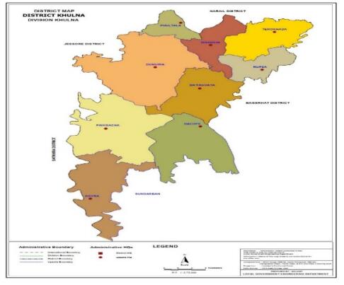 Figure 2. Location of the selected area.
In the data source used, 30 km2 areas were given for the total area of the Upazila including 15 other villages. To make the calculation simple, it has been assumed that all the villages are similar in size. Then the area of the selected village has been found about 2 km2. The condition presented is a typical condition for most of the villages in Bangladesh. There is a significant improvement potential in latrine use and reduction of open defecation but still, people are at risk without any proper wastewater management. The only use of latrines cannot be a single solution, also appropriate wastewater treatment is needed to complete the process and make a healthy environment. In Tables 3 and 4, an approximated estimation of Khulna's water consumption per capita along with source wise consumption has been done using available data provided by KWASA.
| Calculation of Served Population | Numbers (Approximated) | Remarks |
| KWASA's Tube Wells | ||
| 1. Registered Connections 2. Inactive 3. Active 4. Consumers per each 5. Served Population |
15000 2579 12672 13.5 171100 |
(Registered—Inactive) (Active X Consumers per each) |
| Street Hydrant | ||
| 6 Total 7. Inactive 8. Active 9. Consumers per each 10. Served Population |
503 403 100 100 10000 |
(Total—Inactive) (Active X Consumers per each) |
| KWASA's Hand Pumps | ||
| 11. No. of Deep Hand Pumps 12. No. of Shallow Hand Pumps 13. Consumers per each 14. Served Population |
3748 5538 30 278600 |
(Deep Hand Pumps/Shallow Hand Pumps) X Consumers per each |
| Private Wells | ||
| 15. Total 16. Consumers per each 17. Served Population 18. Uncategorized |
13733 30 412000 85300 |
(Total X Consumers per each) |
DownLoad: CSV| Water source | Use | Remarks |
| KWASA's Tube wells | No. of Consumers: 171,100 + 10,000 = 181,100 Water supply: 30,100 m3/day Loss: 30,100 × 0.40 = 12,040 m3/day Net supply: 30,100 − 12,040 = 18,060 m3/day Non-Domestic: 18,060 × 0.2 = 3,610 m3/day Domestic = 18,060 − 3,610 = 14,450 m3/d LPCD = 14.45 − 1000/181,100 = 80 L/day/person |
Water Loss: 40% (Approximated) |
| KWASA's Hand Pumps | No. of Consumers: 278,600 Water supply: 39,300 m3/day Loss: 39300 × 0.10 = 3,930 m3/day Net supply: 39,300 − 3,930 = 35,370 m3/day Non-Domestic: 35,370 × 0.2 = 7,070 m3/day Domestic = 35,370 − 7,070 = 28,300 m3/d LPCD = 28,300 × 1000/27, 8600 = 102 L/day/person |
Water Loss: 10% (Approximated) |
| Private Pumps | No. of Consumers: 412,000 Water supply: 49,700 m3/day Loss: 49,700 × 0.10 = 4,970 m3/day Net supply: 49,700 − 4,970 = 4, 4730 m3/day Non-Domestic: 4, 4730 × 0.2 = 8,950 m3/day Domestic = 44,730 − 8,950 = 35,780 m3/d LPCD = 35,780 × 1000/412,000 = 87 L/day/person |
Water Loss: 10% (Approximated) |
| Total | No. of Consumers: 957,000 Water supply: 119,100 m3/day Loss: 20,940 m3/day Net supply: 98,160 m3/day Non-Domestic: 19,630 m3/day Domestic = 78,530 m3/d LPCD = 78,530 × 1000/957,000 = 87 L/day/person |
N/A |
DownLoad: CSVA typical survey was done to achieve some important values. The average temperature was 30 ℃. The average pH values ranged approximately 6.5–7.8. The Demand of Oxygen (DO) and ORP results had no such abruptions. Some other very important parameters were noted and those were analyzed with other case reports made on the same topic of interest and our results seemed to be with no significant difference. Table 5 represents the compared results and shows different ranged values of important parameters regarding various types of water based on uses [31].
| Parameters | Domestic | Wastewater storage | Agriculture | Fisheries | Urban Domestic | |
| SS (mg/L) | Avg. Max Min |
10–12 50 < 1 |
14–25 55 < 1 |
7–13 21 6 |
29–40 75 6 |
20–32 100 0.60 |
| TOC (mg/L) | Avg. Max Min |
7–12 16 2–2.5 |
10–19 40 4.4 |
12–15 20 5.5 |
12–15.5 21 5.4 |
10–13 17 4.3 |
| T-N (mg/L) | Avg. Max Min |
1–1.56 2.8 0.3 |
2–3.56 13 0.4 |
0.4–0.72 1.33 0.33 |
1.61 4.67 1.12 |
2.1–3.33 4.3 1.113 |
| T-P (mg/L) | Avg. Max Min |
0.1–0.2 1.1 0.01 |
0.7–1.2 2.77 < 0.03 |
0.013–0.05 0.122 < 0.01 |
0.1–0.223 1.12 0.01 |
0.65–1 1.765 0.01 |
DownLoad: CSVBefore designing the process, some basic parameters have been collected from various sources. Among them, average water consumption in rural areas of Bangladesh was found to be 83.17 liters/person/day [32]. It is a bit lower than the urban water consumption. This could be due to less water availability or poor economic condition. Average daily water consumption Q = 83.17 liters/person/day = 0.083 m3/person/day (Appendix 1) will result in an average daily wastewater flow QD = 87.17 m3/day, where, wastewater flow is assumed to be 85% of daily water consumption. Table 6 includes BOD, TN, N as NH4+ and TP in the daily wastewater flow. It also includes required an amount of BOD, N, and P in the effluent for water use in irrigation. Average BOD5 in the influent is calculated in Appendix. The required BOD value in the effluent is found from Table 6. The required values for nitrogen and phosphorus in the effluent are found from a report named Water Quality for Agriculture. The average amount of TN, N, and TP in the influent is estimated as typical content in municipal wastewater with a minor industrial contribution. Calculations are found in Appendix 1. Table 6 shows concentration in effluents and influents [33].
| Sl. No. | Items | Level-1 (A) | Level-1 (B) | Level-2 | Level-3 |
| 1 | COD (mg/L) | 50 | 60 | 100 | 120 |
| 2 | BOD5 (mg/L) | 10 | 20 | 30 | 60 |
| 3 | SS (mg/L) | 10 | 20 | 30 | 50 |
| 4 | Oil (Animal/vegetable) (mg/L) | 1 | 3 | 5 | 20 |
| 5 | Petroleum (mg/L) | 1 | 3 | 5 | 15 |
| 6 | Ammonia (mg/L) | 15 | 20 | − | − |
| 7 | TP | 0.66 | 1 | 3 | 5 |
| 8 | pH | 6.7 | 6.5 | 7.9 | 8.2 |
| 9 | Colon Bacillus (p/L) | 1000 | 10000 | 10000 | − |
| *Note: Levels denotes various stages of wastewater. | |||||
DownLoad: CSVBOD in the influent is calculated from an empirical equation (Appendix 1), for influent BOD, C0 = 1000 B/QD, BOD contribution per day (B) is assumed to 40 g/capita/day for medium-sized communities.
A primary treatment is needed to make the whole treatment process more efficient and to reduce the organic load in the secondary treatment. A septic tank is one of a common type of primary treatment. Also, anaerobic ponds can also act as a primary treatment tool. Septic tank can be installed in each household or one anaerobic pond can be used for the whole community.
An Indian standard code will be used for the design of the septic tank in "Sundermahal" village. Figure 3 represents recommended the size of septic tanks according to the number of users (Bureau of Indian standards, 1993).
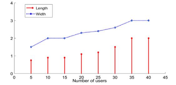 Figure 3. Length and width of septic tank according to the number of users.
If 5 persons in each house are assumed for the selected village, then from Figure 3 the size of a septic tank can be found to be of 1.5 m long and 0.75 m wide. The depth is assumed 1.3 m including 1 m depth from the outlet pipe to the bottom of the tank and 0.3 m distance from roof to liquid. So, a 1.13 m2 septic tank is recommended for each household in this village.
V (volume of septic tank) = (1.5 × 0.75 × 1.3) = 1.46 m3 (approximately).
This septic tank can store 1460 L liquid and each of the houses will need a septic tank of approximately 1.46 m3. Several requirements are stated for installing a septic tank. It should be 60 m away from any community well, 9 m away from any buried water storage tank and 15 m from any source of potable water or natural water body [34,35,36]. A septic tank can remove BOD, TSS, oil, and grease. Typically, a septic tank can remove 30 to 50% BOD and 60 to 80% TSS.
Design of an anaerobic pond below has been done using waste stabilization pond and Constructed Wetland Design Manual:
| Volumeofanaerobicpond,VA=C0QD/λv | (1) |
| Hydraulicretentiontime,tAN=VA/QD | (2) |
From Eq 1, VA = 141 m3 (Appendix 2); for temperature > 25 ℃;
Only a primary treatment is not enough to make the effluent in quality of an acceptable level. With the above design of septic tank and anaerobic pond, 30 to 70% of BOD removal is expected. For secondary treatment different options can be chosen, such as wetland, facultative pond or sand filters. Depending on the geography, landscape and weather condition various options can be adopted.
| Areaoffacultativepond,AF=10C0QD/λ | (3) |
In Bangladesh, the average temperature is assumed to be more than 25 ℃. Here in the calculation 28 ℃ have been used. In this design, a primary treatment has already been suggested. In primary treatment, for septic tank almost 30% BOD is removed. So, in further secondary treatment design, a reduced BOD in the secondary influent is assumed.
From Eq 3, AF = 784.692 m2 (Appendix 3):
| Retentiontime,TF=AFD/QM | (4) |
Where D is the depth of the pond (1.5 m usually) and QM is mean flow, QI is influent flow, QE is effluent flow and "e" is evaporation rate. Evaporation rate for Bangladesh is found from a historical data study and the values vary with temperature during the year. An average monthly evaporation value of 120 mm for 28 ℃ is considered in this calculation [44]. From this, a daily evaporation rate can be calculated. Average daily evaporation rate (e) = 120/30 = 4 mm/day. Let;
| QM=(QI+QE)/2 | (5) |
| QE=QI−0.001AF.e | (6) |
From Eqs 5 and 6, QE = 84 m3/day; QM = 85.67 m3/day = 86 m3/day. Then, putting values of QM and QE in Eq 4, TF = 14 days (approx.) (Appendix 3). Again, if an anaerobic pond is considered as a primary treatment, from the above equation the area for facultative pond becomes 260 m2 and the retention time found 6 days. This variation is because of the high BOD removal in the anaerobic pond, with almost 70% BOD removal in an anaerobic pond.
| Areaofreedbedofwetland,AW=K.QD(lnC0−lnCt) | (7) |
K is a rate constant, the value found for BOD removal K20 = 180 m/year = 0.5 m/day for subsurface wetland and θ is constant and the value is 1.1 [22,23,24,25].
| KT=K20×θ(T−20) | (8) |
K28 = (0.5)×(1.1)28-20 = 1.08 m/day (for 28 ℃)
Using values of K in Eq 7, AW = 346.386 m2 (approx.) (Appendix 4).
This area for subsurface wetland is calculated with 30% BOD reduction from the septic tank. The value varies if an anaerobic pond is used as a pretreatment. Then the area needed will be 209 m2. The depth of the wetland designed above is considered to be 0.6 m. Eqs 7 and 8 have been collected from reference no [38,39,40].
Using guidelines from Washington State Department of Health (2012) and LGED, Bangladesh (2016) an intermitted sand filter is designed below:
| Thesurfaceareaoffilterbed,AS=QD/Loadingrate | (9) |
The maximum loading rate is 2 to 5 gal/day/square feet recommended in the EPA design manual; the depth of media is 46–91 cm [32,33,34,35,36,37,38]. Design loading rate is considered 4 gal/day/square feet. AS = 534.785 m2 (approx.) (Appendix 5). 420 m2 sand filters are found to be suitable for loading rate 4 gal/day/square feet.
The above design shows an overview of the total decentralized system for a typical village. The area of the village is about 2 km2 (assumed). Primary treatment facilities show, occupying a small area of about 37 m2 for the anaerobic pond. For secondary treatment, the area of a wetland found was almost half of the facultative pond. To implement a facultative pond of 784.926 m2 in this small area will not be suitable. In the above design, several systems are discussed with an example size of the treatment facility. Also, a comparison between options has been done to evaluate suitable options according to the situation. To make the effluent reusable; required BOD value has been calculated according to the requirements given by the government in Table 6. As nutrient concentration is important for reusing the effluent water in irrigation, nitrogen and phosphorus removal has been discussed. With a facultative pond, the effluent fulfills requirement given in Table 2. But for the other two systems, N and P concentration was higher than the requirement.
From studies it has been seen that de-centralized wastewater managements have very high potential on nitrogen and phosphorus removal. A normal series of wetland and facultative pond can remove almost 70% of N and 55–60% of P [41,42]. Normally, P removal is proportional to atmospheric temperature. If the designed plant above has an efficiency of 65% (assumed) in both N and P removal then the effluent amount will be 8.1 mg/L and 1.5 mg/L respectively. From Tables 2, 4 and 5 the values seem to be effective. Further analysis on N and P removal shows that this system can sustain up to 65% of nominal efficiency and the wetland along with sand filter can totally can remove up to 21.2 mg/L of N and 11.9 mg/L of P.
De-centralized management system for wastewater treatment has been briefly discussed in this paper and a design has been made regarding economy and environment of Bangladesh. Here, a technical and operational feasibility will be discussed. To apply this system on Bangladesh the first hindrance is local acceptability and govt. funding. USA and Sweden have already applied and made great success on this type of wastewater treatment technologies for their urban domestics. Recently, China applied this technology and they also found great after results. Bangladesh and China have almost same type of environment and soil mostly on every part. So, to apply de-centralize wastewater treatment for Bangladesh it is highly recommended to follow China's plan on DWWT implementation [43,44]. Figure 3 shows the tabular schematic about implementing DWWT in Bangladesh.
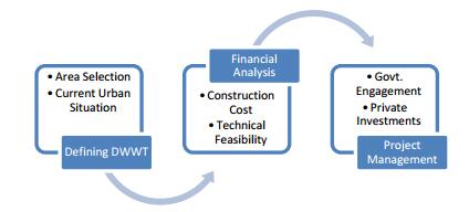 Figure 3. Structure of proposed method.
Feasibility analysis is usually done to see if the system is compatible with the environment or not. Installation and running cost is also analyzed in this section. Mathematically:
| Nk=∑ni{TPi×Ri×WUi+TPi×(1−Ri)×WUNi}×365×Ck×α÷109 | (10) |
| TW=∑niTPFi×WUi×α÷1000 | (11) |
Here,
Nk = total emission of pollutant "k" in kilo-tons/day (where, k1 = COD, k2 = BOD5);
TW = total domestic wastewater emission from small towns and villages in a year "n" in kilo-tons/day;
Ri = ratio of served population within supply area "I" in %;
WUNi = per person water consumption within supply area "I" in L/d;
Ck = concentration of pollutant in domestic waste, mg/L;
A = proportion of waste discharge to water consumption;
TPFi = total population in the area "i" in the year "n" in per thousands.
Here,
| TPFi=TPi×(1+Rp)6 | (12) |
Where, Rp = Avg. growth of population, %.
Below Table 7 shows the approximated rate of wastewater discharge in Khulna from the equations stated above.
| Area | Wastewater from Upazila (Small towns) (kilo-tons/day) | Wastewater from villages (kilo-tons/day) | Total (kilo-tons/day) |
| Phultola | 8000.9 | 200 | 8200.9 |
| Digholia | 1204.33 | 430 | 1634.33 |
| Terokhadia | 3747.853 | 124 | 3871.853 |
| Paikgacha | 2300 | 7200 | 9500 |
| Dumuria | 1366.9 | 9335.777 | 10702.677 |
| Rupsha | 7300 | 35 | 7335 |
| Koyra | 22 | 3750 | 3772 |
| Dakope | 12.5 | 7400 | 7412.5 |
| Batiyaghata | 1430.3 | 8337 | 9767.3 |
| Total: | 62196.56 |
DownLoad: CSVTo analyze the impact on environment, estimation of pollutant reduction plays a very important role. If establishing a new system cannot control pollutant emission then the system will not be feasible for environment. So, estimating the amount of pollution reduction is very important. Mathematically it can be denoted as:
| TRk=TWn×Ck×365×r/TWn×Ck×365×r106106 |
(13[ |
Where, TRk → total reduction of pollutant "k" in kilo-tons per year;
TWn → total amount of domestic wastewater in the year "n" in kilo-tons = 62196.56 kilo-tons/day;
R → treatment percentile ratio in "%" = 40% (can be upgraded to 80%) [47];
Ck → concentration of pollutant "k" in mg/L = 20 – 100 mg/L [38,42,43,44].
If results seem positive and has a satisfactory ration between each then the system can be said to be environment friendly. In our designed system, from Eq 13, the result is approximately 90806.9776 kilo-tons/year, which is a huge reduction rate. Capacity of single unit treatment plant = 10000 tons/day [27,28,29,30,31,32,33,34,35,36,37,38]. Total needed plants in Khulna district = TRk ÷ (365 × Capacity of unit treatment plant)= 90806977.6/(365 × 10000) = 25 (approx.). So, each upazilla will need 25/9 = 3 treatment plants, which will be of the same unit sized.
In this section, financial issues about DWWT development are discussed. Financial demand and pressure for DWWT construction in each upazila area is estimated below along with recommendations on financial structure are provided. At last, operation cost of DWWT facility and the local residents' payment capacity has been analyzed.
The cost demand of DWWT construction in each basin area is calculated by the following formula:
| M=TWn×p×r/1000 | (14) |
In which:
M → cost for construction of DWWT, million USD;
TWn → amount of domestic wastewater from small towns and villages in a year "n", kilo tons/day;
p → construction cost of unit treatment capacity, USD/(ton/d);
r → target of treatment rate in year "n", %.
As the DWWT definition is not familiar in Bangladesh so the exact construction and maintenance cost cannot be calculated nor any govt. reports regarding this technology has been found. So, for reference, 17 previous project reports from China, USA and Sweden has been studied with treatment capacities below 10000 tons/d built between 1996 and 2007 and their cost estimation techniques were investigated to make a rough assumption on DWWT establishment costing for Bangladesh [45,46,47]. Table 8 shows an estimated cost of unit treatment capacity plant.
| Capacity Tons/day | Wetlands (constructed) | Infiltration (Rapid) | Filtration (Catalytic) | Filtration (Biological) | Activated Sludge | Aerated Lagoon | Total |
| 400–500 | − | − | 257.8 | 120 | − | 135 | 420–550 |
| 500–1000 | 145 | − | 230.55 | − | 433.62 | − | 650 (approx.) |
| 1000–1500 | − | 112 | − | − | − | − | n/a |
| 1500–2000 | 132 | − | − | − | − | − | n/a |
| 2000–2500 | 152 | − | − | 134 | 544.4 | − | 750–1000 |
| 2500–3000 | − | − | − | 144 | − | − | 800–1400 |
| 3000–8000 | 233 | 91 | 267.78 | 1200 | 947.5 | 102 | 2000 (approx.) |
DownLoad: CSVBased on studied projects and reports, the unit construction will vary from 500–2000 USD based on design and utility structures. Our basic designed will approximately cost around 650 USD for primary setup. Considering a possible pipeline expansion cost this system needs minimum 800 USD for construction.
In this section, the operation cost of DWWT facility is estimated according to existing small wastewater treatment projects. Combined with the sewage charge level of urban wastewater treatment and payment capacity of rural residents, the sewage charge policy of DWWT is discussed. Case studies are cited to estimate the operation cost of DWWT [48,49], which includes energy cost (C1), medical cost (C2), labor cost (C3), depreciation cost (C4), heavy repair cost (C5), maintenance cost (C6), management cost (C7) and interest cost (C8). According to relevant design standards [50,51,52]:
| C1=e×d×365 | (15) |
Where, e → daily electricity consumption, kWh/d.
d → electricity price, USD/kWh.
| C2=Q.a.b | (16) |
Here, Q → treatment capacity, ton/d;
a → medical consumption, mg/L;
b → medical price, USD/ton.
| C3=Labor salary×numberof labors | (17) |
| C4=originalvalueoffixedassets×depreciationrate | (18) |
| C5=originalvalueoffixedassets×heavyrepairrate | (19) |
| C6=originalvalueoffixedassets×maintenancerate | (20) |
| C7=(C1+C2+C3+C4+C5+C6)×15% | (21) |
| C8=totaldebt×annualinterestrate | (22) |
| Totalcost,TC=C1+C2+C3+C4+C5+C6+C7+C8 | (23) |
| cUnittreatmentcost,UC=TCΣQ | (24) |
In which, ΣQ is the total amount of treated wastewater. The depreciation rate is 5% (equipment 5.33%, sewage pipeline 3.2%, automatic control equipment 9.6%, main structure 3.2%), heavy repair rate is 2%, and maintenance rate 1% [42,43,44,45,46,47,48,49,50,51,52]. Each financial channel has its potential role and possible problems when used in DWWT. Therefore, a multiple financial structure is recommended so that various financial channels could be complementary to each other. The suggestions in previous sections provide basic principles on choice of financial structure with regard to local economic conditions. However, further research based on detailed information of each area is required. In the short term, local residents in rural areas will not be able to pay for the full operation cost of wastewater treatment. Subsidy from local government is strongly required to maintain satisfied operation of the DWWT facilities.
The new wastewater treatment plant is discussed and designed in this paper which is very much cost effective. The plant is easy to make and it treats the water by removing waste from it especially BOD, Nitrogen, and phosphorus. It can be implemented in not only rural areas but also in semi-urban areas. It does not need any modern machinery rather it can be build using very low initial investment comparing to other centralized and de-centralized methods. Any big family or small two to four families can easily use one plant for water treatment. In the above design, some assumptions have been done for various parameters for calculation. In some cases, assumptions may not be similar to reality. Also, the temperature has been considered as 28 ℃, which may be a bit lower than the real situation. This is considered to make the calculation simple. Chosen area is considered as a typical village, but there are areas with different topography than the designed one. So, this design may not be appropriate for hilly or coastal regions in the southern and southwest part of Bangladesh. Nitrogen and phosphorus removal for the designed system has been calculated with a rough estimation. The efficiency could be different in the practical case. This design is an example and a model of the recommended solution. When implementing this solution, in reality, some changes according to necessity could be done. Such as for places with a high groundwater table, depth of anaerobic pond or septic tank could be adjusted. In addition, some specific value of the area of this village has not been found. Therefore, an estimation and assumption have been done. pH of the total system was assumed to be in between 6.5–7, which in real case may differ a little. TDS and arsenic were not considered here to be much severe because the area of design has a very few rates of arsenic and TDS in the ground level. So, those were assumed as constants. If necessary funds can be generated then this project can be investigated further in a big scale.
Nowadays, clean drinking water is one of the crying needs of the general wellbeing of Bangladesh. Every now and then the drinking water quality is greatly hampered due to natural disasters or different man-made deeds. In this paper, a new type of decentralized low-cost water treatment plant is designed considering all the important parameters for implementing in rural regions of Bangladesh. The plant is very much cost effective and the running and operating costs are comparatively low. The plant is well suited for 3 or 4 small families in the village area. Finally, it is interesting to mention some future recommendations related to this research work:
(1) In this paper, the plant is designed for Bangladesh taking Khulna as a standard district. The climatic conditions for different places are different. So, in case of designing the plant for other districts the climatic conditions must be taken into account.
(2) In this design, no special treatment for pathogens are considered, though septic tank and secondary facilities are capable of removing 70% of pathogens. In future research, treatment of pathogens must be considered.
The authors would like to acknowledge LGED, PWD, KWASA and Bangladesh Bureau of Statistics and Bangladesh Meteorological Dept. for providing necessary data and help in conducting the research. The authors would also like to thank all the teachers of Dept. of Mechanical Engineering of Rajshahi University of engineering & Technology and all the respected stuffs of Thermal Engineering Lab. of RUET.
The authors declare no conflict of interest.
| Appendix | Parameter | Unit | Equation | Result |
| 1. Water flow and BOD | Q QD B C0 |
m3/person/d m3/person/d g/capita g/m3 |
N/A % of wastewater flow.Q N/A B/QD |
0.083 87.17 40 565.8 |
| 2. Anaerobic Pond | λv VA tAN |
g/m3/day m3 day |
N/A C0QD/λv 𝑉A/𝑄D |
350 141 1.6 |
| 3. Facultative Pond (30% BOD removal) | λv(T = 28 0C) AF D QE QM TF |
kg/ha.day m2 m m3/day m3/day day |
20T-120 10C0QD/λv N/A QI—0.001AF.e [As, QD = QI] (QI + QE)/2 AFD/QM |
440 784.926 1.5 84 86 14 |
| 4. Wetland | θ K20 KT [T = 28 0C] C0 CT AW |
constant m/day m/day constant constant m2 |
N/A N/A K20.θ(T-20) N/A N/A KQD (ln C0 − ln CT) |
1.1 0.5 1.08 396.2 10 345.386 |
| 5. Sand Filter | Load Rating AS |
L/day/m2 m2 |
N/A QD/Loading Rate |
163 534.785 |
DownLoad: CSV| [1] | F. Brauer, C. Castillo-Chavez, Mathematical models in population biology and epidemiology, New York: Springer, 2 (2012). |
| [2] |
K. Dietz, J. A. Heesterbeek, Daniel Bernoulli's epidemiological model revisited, Math. Biosci., 180 (2002), 1–21. doi: 10.1016/S0025-5564(02)00122-0

|
| [3] | W. O. Kermack, A. G. McKendrick, A contribution to the mathematical theory of epidemics, Proc. R. Soc. Lond. A Math. Phys. Sci., 115 (1927), 700–721. |
| [4] | H. W. Hethcote, The mathematics of infectious diseases, SIAM Rev. Soc. Ind. Appl. Math., 42 (2000), 599–653. |
| [5] | R. M. Anderson, B. Anderson, R. M. May, Infectious diseases of humans: dynamics and control, Oxford University Press, 1992. |
| [6] |
S. Ruan, W. Wang, Dynamical behavior of an epidemic model with a nonlinear incidence rate, J. Differ. Equ., 188 (2003), 135–163. doi: 10.1016/S0022-0396(02)00089-X
|
| [7] |
J. P. Tripathi, S. Abbas, Global dynamics of autonomous and nonautonomous SI epidemic models with nonlinear incidence rate and feedback controls, Nonlinear Dyn, 86 (2016), 337–351. doi: 10.1007/s11071-016-2892-0
|
| [8] | L. J. Gross, Mathematical models in plant biology: An overview, Applied Mathematical Ecology, (1989), 385–407. |
| [9] |
W. M. Liu, H. W. Hethcote, S. A. Levin, Dynamical behavior of epidemiological models with nonlinear incidence rates, J. Math. Biol., 25 (1987), 359–380. doi: 10.1007/BF00277162
|
| [10] |
Y. Cai, Y. Kang, M. Banerjee, W. Wang, A stochastic SIRS epidemic model with infectious force under intervention strategies, J. Differ. Equ., 259 (2015), 7463–7502. doi: 10.1016/j.jde.2015.08.024
|
| [11] |
M. Zhou, T. Zhang, Global Analysis of an SEIR Epidemic Model with Infectious Force under Intervention Strategies, J. Appl. Math. Phys., 7 (2019), 1706. doi: 10.4236/jamp.2019.78117
|
| [12] |
J. Cui, Y. Sun, H. Zhu, The impact of media on the control of infectious diseases, J. Dyn. Differ. Equ., 20 (2008), 31–53. doi: 10.1007/s10884-007-9075-0
|
| [13] | J.A. Cui, X. Tao, H. Zhu, An SIS infection model incorporating media coverage, Rocky Mt. J. Math., (2008), 1323–1334. |
| [14] |
D. Xiao, S. Ruan, Global analysis of an epidemic model with nonmonotone incidence rate, Math. Biosci., 208 (2007), 419–429. doi: 10.1016/j.mbs.2006.09.025
|
| [15] |
Y. Xiao, T. Zhao, S. Tang, Dynamics of an infectious diseases with media/psychology induced non-smooth incidence, Math. Biosci. Eng., 10 (2013), 445. doi: 10.3934/mbe.2013.10.445
|
| [16] |
S. Tang, Y. Xiao, L. Yuan, R. A. Cheke, J. Wu, Campus quarantine (Fengxiao) for curbing emergent infectious diseases: Lessons from mitigating A/H1N1 in Xi'an, China, J. Theor. Biol., 295 (2012), 47–58. doi: 10.1016/j.jtbi.2011.10.035
|
| [17] |
Y. Xiao, S. Tang, J. Wu, Media impact switching surface during an infectious disease outbreak, Sci. Rep., 5 (2015), 7838. doi: 10.1038/srep07838
|
| [18] |
A. B. Gumel, S. Ruan, T. Day, J. Watmough, F. Brauer, P. Van den Driessche, et al., Modelling strategies for controlling SARS outbreaks, Proc. R. Soc. Lond. B Biol. Sci., 271 (2004), 2223–2232. doi: 10.1098/rspb.2004.2800
|
| [19] | J. Zhang, J. Lou, Z. Ma, J. Wu, A compartmental model for the analysis of SARS transmission patterns and outbreak control measures in China, Appl. Math. Comput., 162 (2005), 909–924. |
| [20] |
S. Bugalia, V. P. Bajiya, J. P. Tripathi, M. T. Li, G. Q. Sun, Mathematical modeling of COVID-19 transmission: The roles of intervention strategies and lockdown, Math. Biosci. Eng., 17 (2020), 5961–5986. doi: 10.3934/mbe.2020318
|
| [21] |
V. P. Bajiya, S. Bugalia, J. P. Tripathi, Mathematical modeling of COVID-19: Impact of non-pharmaceutical interventions in India, Chaos Interdiscipl. J. Nonlinear Sci., 30 (2020), 113143. doi: 10.1063/5.0021353
|
| [22] |
M. T. Li, G. Q. Sun, J. Zhang, Y. Zhao, X. Pei, L. Li, et al., Analysis of COVID-19 transmission in Shanxi Province with discrete time imported cases, Math. Biosci. Eng., 17 (2020), 3710. doi: 10.3934/mbe.2020208
|
| [23] |
C. N. Ngonghala, E. Iboi, S. Eikenberry, M. Scotch, C. R. MacIntyre, M. H. Bonds, et al., Mathematical assessment of the impact of non-pharmaceutical interventions on curtailing the 2019 novel Coronavirus, Math. Biosci., 325 (2020), 108364. doi: 10.1016/j.mbs.2020.108364
|
| [24] | S. Batabyal, A. Batabyal, Mathematical computations on epidemiology: A case study of the novel coronavirus (SARS-CoV-2), Theory Biosci., (2021), 1–16. |
| [25] |
S. Batabyal, COVID-19: Perturbation dynamics resulting chaos to stable with seasonality transmission, Chaos Solitons Fractals, 145 (2021), 110772. doi: 10.1016/j.chaos.2021.110772
|
| [26] |
W. Wang, S. Ruan, Bifurcations in an epidemic model with constant removal rate of the infectives, J. Math. Anal. Appl., 291 (2004), 775–793. doi: 10.1016/j.jmaa.2003.11.043
|
| [27] |
W. Wang, Epidemic models with nonlinear infection forces, Math. Biosci. Eng., 3 (2006), 267. doi: 10.3934/mbe.2006.3.267
|
| [28] |
C. Shan, H. Zhu, Bifurcations and complex dynamics of an SIR model with the impact of the number of hospital beds, J. Differ. Equ., 257 (2014), 1662–1688. doi: 10.1016/j.jde.2014.05.030
|
| [29] |
G. H. Li, Y. X. Zhang, Dynamic behaviors of a modified SIR model in epidemic diseases using nonlinear incidence and recovery rates, PLoS One, 12 (2017), e0175789. doi: 10.1371/journal.pone.0175789
|
| [30] |
R. Mu, A. Wei, Y. Yang, Global dynamics and sliding motion in A (H7N9) epidemic models with limited resources and Filippov control, J. Math. Anal. Appl., 477 (2019), 1296–1317. doi: 10.1016/j.jmaa.2019.05.013
|
| [31] |
H. Zhao, L. Wang, S. M. Oliva, H. Zhu, Modeling and Dynamics Analysis of Zika Transmission with Limited Medical Resources, Bull. Math. Biol., 82 (2020), 1–50. doi: 10.1007/s11538-019-00680-3
|
| [32] | A. Sirijampa, S. Chinviriyasit, W. Chinviriyasit, Hopf bifurcation analysis of a delayed SEIR epidemic model with infectious force in latent and infected period, Adv. Differ. Equ., 1 (2018), 348. |
| [33] |
E. Beretta, D. Breda, An SEIR epidemic model with constant latency time and infectious period, Math. Biosci. Eng., 8 (2011), 931. doi: 10.3934/mbe.2011.8.931
|
| [34] |
Z. Zhang, S. Kundu, J. P. Tripathi, S. Bugalia, Stability and Hopf bifurcation analysis of an SVEIR epidemic model with vaccination and multiple time delays, Chaos Solitons Fractals, 131 (2020), 109483. doi: 10.1016/j.chaos.2019.109483
|
| [35] |
P. Song, Y. Xiao, Global hopf bifurcation of a delayed equation describing the lag effect of media impact on the spread of infectious disease, J. Math. Biol., 76 (2018), 1249–1267. doi: 10.1007/s00285-017-1173-y
|
| [36] |
A. K. Misra, A. Sharma, V. Singh, Effect of awareness programs in controlling the prevalence of an epidemic with time delay, J. Biol. Sys., 19 (2011), 389–402. doi: 10.1142/S0218339011004020
|
| [37] |
F. Al Basir, S. Adhurya, M. Banerjee, E. Venturino, S. Ray, Modelling the Effect of Incubation and Latent Periods on the Dynamics of Vector-Borne Plant Viral Diseases, Bull. Math. Biol., 82 (2020), 1–22. doi: 10.1007/s11538-019-00680-3
|
| [38] |
S. Liao, W. Yang, Cholera model incorporating media coverage with multiple delays, Math. Methods Appl. Sci., 42 (2019), 419–439. doi: 10.1002/mma.5175
|
| [39] |
K. A. Pawelek, S. Liu, F. Pahlevani, L. Rong, A model of HIV-1 infection with two time delays: mathematical analysis and comparison with patient data, Math. Biosci., 235 (2012), 98–109. doi: 10.1016/j.mbs.2011.11.002
|
| [40] | D. Greenhalgh, S. Rana, S. Samanta, T. Sardar, S. Bhattacharya, J. Chattopadhyay, Awareness programs control infectious disease–multiple delay induced mathematical model, Appl. Math. Comput., 251 (2015), 539–563. |
| [41] |
H. Zhao, M. Zhao, Global Hopf bifurcation analysis of an susceptible-infective-removed epidemic model incorporating media coverage with time delay, J. Biol. Dyn., 11 (2017), 8–24. doi: 10.1080/17513758.2016.1229050
|
| [42] | F. Al Basir, S. Ray, E. Venturino, Role of media coverage and delay in controlling infectious diseases: A mathematical model, Appl. Math. Comput., 337 (2018), 372–385. |
| [43] |
J. Liu, Bifurcation analysis for a delayed SEIR epidemic model with saturated incidence and saturated treatment function, J. Biol. Dyn., 13 (2019), 461–480. doi: 10.1080/17513758.2019.1631965
|
| [44] |
G. H. Li, Y. X. Zhang, Dynamic behaviors of a modified SIR model in epidemic diseases using nonlinear incidence and recovery rates, PLoS One, 12 (2017), e0175789. doi: 10.1371/journal.pone.0175789
|
| [45] | D. P. Gao, N. J. Huang, S. M. Kang, C. Zhang, Global stability analysis of an SVEIR epidemic model with general incidence rate, Bound. Value Probl., (2018), 42. |
| [46] |
G. Huang, Y. Takeuchi, W. Ma, D. Wei, Global stability for delay SIR and SEIR epidemic models with nonlinear incidence rate, Bull. Math. Biol., 72 (2010), 1192–1207. doi: 10.1007/s11538-009-9487-6
|
| [47] |
E. Beretta, Y. Kuang, Geometric stability switch criteria in delay differential systems with delay dependent parameters, SIAM J. Math. Anal., 33 (2002), 1144–1165. doi: 10.1137/S0036141000376086
|
| [48] |
Q. An, E. Beretta, Y. Kuang, C. Wang, H. Wang, Geometric stability switch criteria in delay differential equations with two delays and delay dependent parameters, J. Differ. Equ., 266 (2019), 7073–7100. doi: 10.1016/j.jde.2018.11.025
|
| [49] | Y. Kuang, editor, Delay differential equations: with applications in population dynamics, Academic Press, 1993. |
| [50] |
X. Yang, Generalized form of Hurwitz-Routh criterion and Hopf bifurcation of higher order, Appl. Math. Lett., 15 (2002), 615–621. doi: 10.1016/S0893-9659(02)80014-3
|
| [51] |
C. Castillo-Chavez, B. Song, Dynamical models of tuberculosis and their applications, Math. Biosci. Eng., 1 (2004), 361. doi: 10.3934/mbe.2004.1.361
|
| [52] | C. Castillo-Chavez, Z. Feng, W. Huang, On the computation of R0 and its role on global stability, IMA Volumes in Mathematics and Its Applications, 1 (2002), 229. |
| [53] | Y. Y. Min, Y. G. Liu, Barbalat lemma and its application in analysis of system stability, Journal of Shandong University (engineering science), 37 (2007), 51–55. |
| [54] | S. Ruan, J. Wei, On the zeros of transcendental functions with applications to stability of delay differential equations with two delays, Dynamics of Continuous Discrete and Impulsive Systems Series A, 10 (2003), 863–874. |
| [55] |
H. L. Freedman, V. S. Rao, The trade-off between mutual interference and time lags in predator-prey systems, Bull. Math. Biol., 45 (1983), 991–1004. doi: 10.1016/S0092-8240(83)80073-1
|
| [56] |
L. H. Erbe, H. I. Freedman, V. S. Rao, Three-species food-chain models with mutual interference and time delays, Math. Biosci., 80 (1986), 57–80. doi: 10.1016/0025-5564(86)90067-2
|
| [57] | B. D. Hassard, N. D. Kazarinoff, Y. H. Wan, Y. W. Wan, Theory and applications of Hopf bifurcation, CUP Archive, 41 (1981). |
| [58] | J. J. Benedetto, W. Czaja, Riesz Representation Theorem, In Integration and Modern Analysis, Birkhäuser Boston, (2009), 321–357. |
| [59] |
J. Wu, Symmetric functional differential equations and neural networks with memory, Trans. Am. Math. Soc., 350 (1998), 4799–4838. doi: 10.1090/S0002-9947-98-02083-2
|
| [60] |
H. I. Freedman, S. Ruan, M. Tang, Uniform persistence and flows near a closed positively invariant set, J. Dyn. Differ. Equ., 6 (1994), 583–600. doi: 10.1007/BF02218848
|
| [61] | Worldometer, coronavirus, available from: https://www.worldometers.info/coronavirus/. |
| [62] | The print news, available from: https://theprint.in/world/this-is-how-france\-italy-and-spain-are-easing-their-lockdowns-one-step-at-a-time/413060/. |
| [63] | World Health Organization, COVID-19. Available from: https://covid19.who.int/. |
| [64] | X. Lin, H. Wang, Stability analysis of delay differential equations with two discrete delays, Canadian Appl. Math. Quart., 20 (2012), 519–533. |
| [65] |
L. Wang, J. Wang, H. Zhao, Y. Shi, K. Wang, P. Wu, et al., Modelling and assessing the effects of medical resources on transmission of novel coronavirus (COVID-19) in Wuhan, China, Math. Biosci. Eng., 17 (2020), 2936–2949. doi: 10.3934/mbe.2020165
|
| 1. | Kayden KM Low, Maurice HT Ling, 2024, 9780128096338, 10.1016/B978-0-323-95502-7.00105-6 |


Figures(29) / Tables(4)

Sarita Bugalia, Jai Prakash Tripathi, Hao Wang. Mathematical modeling of intervention and low medical resource availability with delays: Applications to COVID-19 outbreaks in Spain and Italy[J]. Mathematical Biosciences and Engineering, 2021, 18(5): 5865-5920. doi: 10.3934/mbe.2021295

| Sl. No. | Water Quality Parameters |
Bangladesh Standards (mg/L) | WHO Guide Line |
Methods/Equipment |
| 01 | Aluminum | 0.2 | − | Atomic Absorption Apectro-photometer (AAS) |
| 02 | Ammonia | 0.5 | UV-VIS | |
| 03 | Arsenic | 0.05 | 0.01 | AAS |
| 04 | Barium | 0.01 | 0.7 | AAS |
| 05 | Benzene | 0.01 | 0.01 | Gas Chromatograph |
| 06 | BOD 5 day, 20 ℃ | 0.2 | − | 5 days Incubation |
| 07 | Boron | 1.0 | − | UV-VIS |
| 08 | Cadmium | 0.005 | 0.003 | AAS |
| 09 | Calcium | 75 | − | AAS |
| 10 | Chloride | 150–600 | − | Titrimetric |
| 11 | Chlorinated Alkenes | |||
| 11.1 | Carbontetrachloride | 0.01 | 0.004 | Gas Chromatograph |
| 11.2 | 1.1 DichloroEthelene | 0.001 | 0.03 | Gas Chromatograph |
| 11.3 | 1.2 DichloroEthelene | 0.03 | 0.03 | Gas Chromatograph |
| 11.4 | TetrachloroEthelene | 0.03 | 0.04 | Gas Chromatograph |
| 11.5 | TrichloroEthelene | 0.09 | 0.07 | Gas Chromatograph |
| 12.1 | Pentachlorophenol | 0.03 | 0.009 | Gas Chromatograph |
| 12.2 | 2, 4, 6-Trichlorophenol | 0.03 | 0.2 | Gas Chromatograph |
| 13 | Chlorine (Residual) | 0.2 | − | Titrimetric |
| 14 | Chloroform | 0.09 | 0.2 | Gas Chromatograph |
| 15 | Chromium (Hexavalent) | 0.05 | − | Iron Chromatograph |
| 16 | Chromium (Total) | 0.05 | 0.05 (P) | AAS |
| 17 | COD | 4 | − | Closed Reflux Method |
| 18 | Coli form (Fecal) | 0 CFU (N/100 mL) | 0 | Membrane Filtration Method |
| 19 | Coli form (Total) | 0 CFU (N/100 mL) | 0 | Membrane Filtration Method |
| 20 | Color | 15 Hazen | − | Color Comparator |
| 21 | Copper | 1 | 2 | AAS |
| 22 | Cyanide | 0.1 | 0.07 | UV-VIS/Specific Ion Electrode |
| 23 | Detergent | 0.2 | − | UV-VIS |
| 24 | DO | 6 | − | Multimeter |
| 25 | Electric Conductivity | −us/cm | − | Multimeter |
| 26 | Fluoride | 1 | 1.5 | UV-VIS |
| 27 | Hardness as CaCO3 | 200–500 | − | Titrimetric |
| 28 | Iodine | 200–500 | − | Titrimetric |
| 29 | Iron | 0.3–1.0 | − | AAS |
| 30 | Nitrogen (Total) | 1 | − | UV-VIS/Digestion |
| 31 | Lead | 0.05 | 0.01 | AAS |
| 32 | Magnesium | 30–35 | − | AAS |
| 33 | Manganese | 0.1 | − | AAS |
| 34 | Mercury | 0.001 | 0.001 | Mercury Analyzer |
| 35 | Nickel | 0.1 | 0.02 (P) | AAS |
| 36 | Nitrate | 10 | 50.0 as N | UV-VIS |
| 37 | Nitrite | < 1 | 3.0 (0.2) | UV-VIS |
| 38 | Odor | Odorless | − | Threshold Method |
| 39 | ORP (Eh) | − | − | ORP meter |
| 40 | Oil and Grease | 0.01 | − | Oil and Grease meter |
| 41 | pH | 6.5–8.5 | pH Meter | |
| 42 | Phenolic Compounds | 0.002 | − | Gas Chromatograph |
| 43 | Phosphate | 6 | − | UV-VIS |
| 44 | Phosphorus | 0 | − | Digestion |
| 45 | Potassium | 12 | − | AAS |
| 46 | Radioactive Materials (Gross Alpha Activity) | 0.01 Bq/L | 0.5 Bq/L | − |
| 47 | Radioactive Materials (Gross Beta Activity) | 0.1 Bq/L | 1.0 Bq/L | − |
| 48 | Salinity | − | − | Multimeter |
| 49 | Selenium | 0.01 | 0.01 | AAS |
| 50 | Silver | 0.02 | − | AAS |
| 51 | Sodium | 200 | − | AAS |
| 52 | Suspended Solids | 10 | − | Filtration and Drying |
| 53 | Sulphide | 0 | − | UV-VIS |
| 54 | Sulphate | 400 | − | UV-VIS |
| 55 | Taste | − | − | Threshold Method |
| 56 | Total Alkalinity | − | − | Titrimetric |
| 57 | Total Dissolved Solid | 1000 | − | Multimeter |
| 58 | Temperature | 20–30 C | Thermometer | |
| 59 | Tin | 2 | − | AAS |
| 60 | Turbidity | 10 NTU | − | Turbidity meter |
| 61 | Zinc | 5 | − | AAS |
DownLoad: CSV| Parameter | Irrigation | Agriculture | Drinking | Treated Values |
| pH | 6–8.73 | 6.00–8 | 6.5–8.5 | 6–6.5 |
| EC (Us/m) | 0–3.00 | 0.20–0.25 | 0.25 | 0.3–0.4 |
| DO (ppm) | 4.25–5 | 5 | 3.5–5 | 3–4.8 |
| TDS (ppm) | 0–1900 | 150 | 450–510 | 350–420 |
| Total Nitrogen (ppm) | 0–32.00 | 0–0.1 | 1 | 4–4.9 |
| Phosphorus (ppm) | 0–2 | 0–0.1 | N/A | 9.8–10 |
| Cadmium (ppm) | 0–0.0125 | 0.25–1.8 | 0–0.002 | 0 |
| Iron (ppm) | 3.5–5.00 | 0.2 | 0–0.068 | 1.5–1.75 |
| Manganese (ppm) | 0–0.22 | 0–0.009 | 0–0.02 | 0.15 |
DownLoad: CSV| Calculation of Served Population | Numbers (Approximated) | Remarks |
| KWASA's Tube Wells | ||
| 1. Registered Connections 2. Inactive 3. Active 4. Consumers per each 5. Served Population |
15000 2579 12672 13.5 171100 |
(Registered—Inactive) (Active X Consumers per each) |
| Street Hydrant | ||
| 6 Total 7. Inactive 8. Active 9. Consumers per each 10. Served Population |
503 403 100 100 10000 |
(Total—Inactive) (Active X Consumers per each) |
| KWASA's Hand Pumps | ||
| 11. No. of Deep Hand Pumps 12. No. of Shallow Hand Pumps 13. Consumers per each 14. Served Population |
3748 5538 30 278600 |
(Deep Hand Pumps/Shallow Hand Pumps) X Consumers per each |
| Private Wells | ||
| 15. Total 16. Consumers per each 17. Served Population 18. Uncategorized |
13733 30 412000 85300 |
(Total X Consumers per each) |
DownLoad: CSV| Water source | Use | Remarks |
| KWASA's Tube wells | No. of Consumers: 171,100 + 10,000 = 181,100 Water supply: 30,100 m3/day Loss: 30,100 × 0.40 = 12,040 m3/day Net supply: 30,100 − 12,040 = 18,060 m3/day Non-Domestic: 18,060 × 0.2 = 3,610 m3/day Domestic = 18,060 − 3,610 = 14,450 m3/d LPCD = 14.45 − 1000/181,100 = 80 L/day/person |
Water Loss: 40% (Approximated) |
| KWASA's Hand Pumps | No. of Consumers: 278,600 Water supply: 39,300 m3/day Loss: 39300 × 0.10 = 3,930 m3/day Net supply: 39,300 − 3,930 = 35,370 m3/day Non-Domestic: 35,370 × 0.2 = 7,070 m3/day Domestic = 35,370 − 7,070 = 28,300 m3/d LPCD = 28,300 × 1000/27, 8600 = 102 L/day/person |
Water Loss: 10% (Approximated) |
| Private Pumps | No. of Consumers: 412,000 Water supply: 49,700 m3/day Loss: 49,700 × 0.10 = 4,970 m3/day Net supply: 49,700 − 4,970 = 4, 4730 m3/day Non-Domestic: 4, 4730 × 0.2 = 8,950 m3/day Domestic = 44,730 − 8,950 = 35,780 m3/d LPCD = 35,780 × 1000/412,000 = 87 L/day/person |
Water Loss: 10% (Approximated) |
| Total | No. of Consumers: 957,000 Water supply: 119,100 m3/day Loss: 20,940 m3/day Net supply: 98,160 m3/day Non-Domestic: 19,630 m3/day Domestic = 78,530 m3/d LPCD = 78,530 × 1000/957,000 = 87 L/day/person |
N/A |
DownLoad: CSV| Parameters | Domestic | Wastewater storage | Agriculture | Fisheries | Urban Domestic | |
| SS (mg/L) | Avg. Max Min |
10–12 50 < 1 |
14–25 55 < 1 |
7–13 21 6 |
29–40 75 6 |
20–32 100 0.60 |
| TOC (mg/L) | Avg. Max Min |
7–12 16 2–2.5 |
10–19 40 4.4 |
12–15 20 5.5 |
12–15.5 21 5.4 |
10–13 17 4.3 |
| T-N (mg/L) | Avg. Max Min |
1–1.56 2.8 0.3 |
2–3.56 13 0.4 |
0.4–0.72 1.33 0.33 |
1.61 4.67 1.12 |
2.1–3.33 4.3 1.113 |
| T-P (mg/L) | Avg. Max Min |
0.1–0.2 1.1 0.01 |
0.7–1.2 2.77 < 0.03 |
0.013–0.05 0.122 < 0.01 |
0.1–0.223 1.12 0.01 |
0.65–1 1.765 0.01 |
DownLoad: CSV| Sl. No. | Items | Level-1 (A) | Level-1 (B) | Level-2 | Level-3 |
| 1 | COD (mg/L) | 50 | 60 | 100 | 120 |
| 2 | BOD5 (mg/L) | 10 | 20 | 30 | 60 |
| 3 | SS (mg/L) | 10 | 20 | 30 | 50 |
| 4 | Oil (Animal/vegetable) (mg/L) | 1 | 3 | 5 | 20 |
| 5 | Petroleum (mg/L) | 1 | 3 | 5 | 15 |
| 6 | Ammonia (mg/L) | 15 | 20 | − | − |
| 7 | TP | 0.66 | 1 | 3 | 5 |
| 8 | pH | 6.7 | 6.5 | 7.9 | 8.2 |
| 9 | Colon Bacillus (p/L) | 1000 | 10000 | 10000 | − |
| *Note: Levels denotes various stages of wastewater. | |||||
DownLoad: CSV| Area | Wastewater from Upazila (Small towns) (kilo-tons/day) | Wastewater from villages (kilo-tons/day) | Total (kilo-tons/day) |
| Phultola | 8000.9 | 200 | 8200.9 |
| Digholia | 1204.33 | 430 | 1634.33 |
| Terokhadia | 3747.853 | 124 | 3871.853 |
| Paikgacha | 2300 | 7200 | 9500 |
| Dumuria | 1366.9 | 9335.777 | 10702.677 |
| Rupsha | 7300 | 35 | 7335 |
| Koyra | 22 | 3750 | 3772 |
| Dakope | 12.5 | 7400 | 7412.5 |
| Batiyaghata | 1430.3 | 8337 | 9767.3 |
| Total: | 62196.56 |
DownLoad: CSV| Capacity Tons/day | Wetlands (constructed) | Infiltration (Rapid) | Filtration (Catalytic) | Filtration (Biological) | Activated Sludge | Aerated Lagoon | Total |
| 400–500 | − | − | 257.8 | 120 | − | 135 | 420–550 |
| 500–1000 | 145 | − | 230.55 | − | 433.62 | − | 650 (approx.) |
| 1000–1500 | − | 112 | − | − | − | − | n/a |
| 1500–2000 | 132 | − | − | − | − | − | n/a |
| 2000–2500 | 152 | − | − | 134 | 544.4 | − | 750–1000 |
| 2500–3000 | − | − | − | 144 | − | − | 800–1400 |
| 3000–8000 | 233 | 91 | 267.78 | 1200 | 947.5 | 102 | 2000 (approx.) |
DownLoad: CSV| Appendix | Parameter | Unit | Equation | Result |
| 1. Water flow and BOD | Q QD B C0 |
m3/person/d m3/person/d g/capita g/m3 |
N/A % of wastewater flow.Q N/A B/QD |
0.083 87.17 40 565.8 |
| 2. Anaerobic Pond | λv VA tAN |
g/m3/day m3 day |
N/A C0QD/λv 𝑉A/𝑄D |
350 141 1.6 |
| 3. Facultative Pond (30% BOD removal) | λv(T = 28 0C) AF D QE QM TF |
kg/ha.day m2 m m3/day m3/day day |
20T-120 10C0QD/λv N/A QI—0.001AF.e [As, QD = QI] (QI + QE)/2 AFD/QM |
440 784.926 1.5 84 86 14 |
| 4. Wetland | θ K20 KT [T = 28 0C] C0 CT AW |
constant m/day m/day constant constant m2 |
N/A N/A K20.θ(T-20) N/A N/A KQD (ln C0 − ln CT) |
1.1 0.5 1.08 396.2 10 345.386 |
| 5. Sand Filter | Load Rating AS |
L/day/m2 m2 |
N/A QD/Loading Rate |
163 534.785 |
DownLoad: CSV| Sl. No. | Water Quality Parameters |
Bangladesh Standards (mg/L) | WHO Guide Line |
Methods/Equipment |
| 01 | Aluminum | 0.2 | − | Atomic Absorption Apectro-photometer (AAS) |
| 02 | Ammonia | 0.5 | UV-VIS | |
| 03 | Arsenic | 0.05 | 0.01 | AAS |
| 04 | Barium | 0.01 | 0.7 | AAS |
| 05 | Benzene | 0.01 | 0.01 | Gas Chromatograph |
| 06 | BOD 5 day, 20 ℃ | 0.2 | − | 5 days Incubation |
| 07 | Boron | 1.0 | − | UV-VIS |
| 08 | Cadmium | 0.005 | 0.003 | AAS |
| 09 | Calcium | 75 | − | AAS |
| 10 | Chloride | 150–600 | − | Titrimetric |
| 11 | Chlorinated Alkenes | |||
| 11.1 | Carbontetrachloride | 0.01 | 0.004 | Gas Chromatograph |
| 11.2 | 1.1 DichloroEthelene | 0.001 | 0.03 | Gas Chromatograph |
| 11.3 | 1.2 DichloroEthelene | 0.03 | 0.03 | Gas Chromatograph |
| 11.4 | TetrachloroEthelene | 0.03 | 0.04 | Gas Chromatograph |
| 11.5 | TrichloroEthelene | 0.09 | 0.07 | Gas Chromatograph |
| 12.1 | Pentachlorophenol | 0.03 | 0.009 | Gas Chromatograph |
| 12.2 | 2, 4, 6-Trichlorophenol | 0.03 | 0.2 | Gas Chromatograph |
| 13 | Chlorine (Residual) | 0.2 | − | Titrimetric |
| 14 | Chloroform | 0.09 | 0.2 | Gas Chromatograph |
| 15 | Chromium (Hexavalent) | 0.05 | − | Iron Chromatograph |
| 16 | Chromium (Total) | 0.05 | 0.05 (P) | AAS |
| 17 | COD | 4 | − | Closed Reflux Method |
| 18 | Coli form (Fecal) | 0 CFU (N/100 mL) | 0 | Membrane Filtration Method |
| 19 | Coli form (Total) | 0 CFU (N/100 mL) | 0 | Membrane Filtration Method |
| 20 | Color | 15 Hazen | − | Color Comparator |
| 21 | Copper | 1 | 2 | AAS |
| 22 | Cyanide | 0.1 | 0.07 | UV-VIS/Specific Ion Electrode |
| 23 | Detergent | 0.2 | − | UV-VIS |
| 24 | DO | 6 | − | Multimeter |
| 25 | Electric Conductivity | −us/cm | − | Multimeter |
| 26 | Fluoride | 1 | 1.5 | UV-VIS |
| 27 | Hardness as CaCO3 | 200–500 | − | Titrimetric |
| 28 | Iodine | 200–500 | − | Titrimetric |
| 29 | Iron | 0.3–1.0 | − | AAS |
| 30 | Nitrogen (Total) | 1 | − | UV-VIS/Digestion |
| 31 | Lead | 0.05 | 0.01 | AAS |
| 32 | Magnesium | 30–35 | − | AAS |
| 33 | Manganese | 0.1 | − | AAS |
| 34 | Mercury | 0.001 | 0.001 | Mercury Analyzer |
| 35 | Nickel | 0.1 | 0.02 (P) | AAS |
| 36 | Nitrate | 10 | 50.0 as N | UV-VIS |
| 37 | Nitrite | < 1 | 3.0 (0.2) | UV-VIS |
| 38 | Odor | Odorless | − | Threshold Method |
| 39 | ORP (Eh) | − | − | ORP meter |
| 40 | Oil and Grease | 0.01 | − | Oil and Grease meter |
| 41 | pH | 6.5–8.5 | pH Meter | |
| 42 | Phenolic Compounds | 0.002 | − | Gas Chromatograph |
| 43 | Phosphate | 6 | − | UV-VIS |
| 44 | Phosphorus | 0 | − | Digestion |
| 45 | Potassium | 12 | − | AAS |
| 46 | Radioactive Materials (Gross Alpha Activity) | 0.01 Bq/L | 0.5 Bq/L | − |
| 47 | Radioactive Materials (Gross Beta Activity) | 0.1 Bq/L | 1.0 Bq/L | − |
| 48 | Salinity | − | − | Multimeter |
| 49 | Selenium | 0.01 | 0.01 | AAS |
| 50 | Silver | 0.02 | − | AAS |
| 51 | Sodium | 200 | − | AAS |
| 52 | Suspended Solids | 10 | − | Filtration and Drying |
| 53 | Sulphide | 0 | − | UV-VIS |
| 54 | Sulphate | 400 | − | UV-VIS |
| 55 | Taste | − | − | Threshold Method |
| 56 | Total Alkalinity | − | − | Titrimetric |
| 57 | Total Dissolved Solid | 1000 | − | Multimeter |
| 58 | Temperature | 20–30 C | Thermometer | |
| 59 | Tin | 2 | − | AAS |
| 60 | Turbidity | 10 NTU | − | Turbidity meter |
| 61 | Zinc | 5 | − | AAS |
| Parameter | Irrigation | Agriculture | Drinking | Treated Values |
| pH | 6–8.73 | 6.00–8 | 6.5–8.5 | 6–6.5 |
| EC (Us/m) | 0–3.00 | 0.20–0.25 | 0.25 | 0.3–0.4 |
| DO (ppm) | 4.25–5 | 5 | 3.5–5 | 3–4.8 |
| TDS (ppm) | 0–1900 | 150 | 450–510 | 350–420 |
| Total Nitrogen (ppm) | 0–32.00 | 0–0.1 | 1 | 4–4.9 |
| Phosphorus (ppm) | 0–2 | 0–0.1 | N/A | 9.8–10 |
| Cadmium (ppm) | 0–0.0125 | 0.25–1.8 | 0–0.002 | 0 |
| Iron (ppm) | 3.5–5.00 | 0.2 | 0–0.068 | 1.5–1.75 |
| Manganese (ppm) | 0–0.22 | 0–0.009 | 0–0.02 | 0.15 |
| Calculation of Served Population | Numbers (Approximated) | Remarks |
| KWASA's Tube Wells | ||
| 1. Registered Connections 2. Inactive 3. Active 4. Consumers per each 5. Served Population |
15000 2579 12672 13.5 171100 |
(Registered—Inactive) (Active X Consumers per each) |
| Street Hydrant | ||
| 6 Total 7. Inactive 8. Active 9. Consumers per each 10. Served Population |
503 403 100 100 10000 |
(Total—Inactive) (Active X Consumers per each) |
| KWASA's Hand Pumps | ||
| 11. No. of Deep Hand Pumps 12. No. of Shallow Hand Pumps 13. Consumers per each 14. Served Population |
3748 5538 30 278600 |
(Deep Hand Pumps/Shallow Hand Pumps) X Consumers per each |
| Private Wells | ||
| 15. Total 16. Consumers per each 17. Served Population 18. Uncategorized |
13733 30 412000 85300 |
(Total X Consumers per each) |
| Water source | Use | Remarks |
| KWASA's Tube wells | No. of Consumers: 171,100 + 10,000 = 181,100 Water supply: 30,100 m3/day Loss: 30,100 × 0.40 = 12,040 m3/day Net supply: 30,100 − 12,040 = 18,060 m3/day Non-Domestic: 18,060 × 0.2 = 3,610 m3/day Domestic = 18,060 − 3,610 = 14,450 m3/d LPCD = 14.45 − 1000/181,100 = 80 L/day/person |
Water Loss: 40% (Approximated) |
| KWASA's Hand Pumps | No. of Consumers: 278,600 Water supply: 39,300 m3/day Loss: 39300 × 0.10 = 3,930 m3/day Net supply: 39,300 − 3,930 = 35,370 m3/day Non-Domestic: 35,370 × 0.2 = 7,070 m3/day Domestic = 35,370 − 7,070 = 28,300 m3/d LPCD = 28,300 × 1000/27, 8600 = 102 L/day/person |
Water Loss: 10% (Approximated) |
| Private Pumps | No. of Consumers: 412,000 Water supply: 49,700 m3/day Loss: 49,700 × 0.10 = 4,970 m3/day Net supply: 49,700 − 4,970 = 4, 4730 m3/day Non-Domestic: 4, 4730 × 0.2 = 8,950 m3/day Domestic = 44,730 − 8,950 = 35,780 m3/d LPCD = 35,780 × 1000/412,000 = 87 L/day/person |
Water Loss: 10% (Approximated) |
| Total | No. of Consumers: 957,000 Water supply: 119,100 m3/day Loss: 20,940 m3/day Net supply: 98,160 m3/day Non-Domestic: 19,630 m3/day Domestic = 78,530 m3/d LPCD = 78,530 × 1000/957,000 = 87 L/day/person |
N/A |
| Parameters | Domestic | Wastewater storage | Agriculture | Fisheries | Urban Domestic | |
| SS (mg/L) | Avg. Max Min |
10–12 50 < 1 |
14–25 55 < 1 |
7–13 21 6 |
29–40 75 6 |
20–32 100 0.60 |
| TOC (mg/L) | Avg. Max Min |
7–12 16 2–2.5 |
10–19 40 4.4 |
12–15 20 5.5 |
12–15.5 21 5.4 |
10–13 17 4.3 |
| T-N (mg/L) | Avg. Max Min |
1–1.56 2.8 0.3 |
2–3.56 13 0.4 |
0.4–0.72 1.33 0.33 |
1.61 4.67 1.12 |
2.1–3.33 4.3 1.113 |
| T-P (mg/L) | Avg. Max Min |
0.1–0.2 1.1 0.01 |
0.7–1.2 2.77 < 0.03 |
0.013–0.05 0.122 < 0.01 |
0.1–0.223 1.12 0.01 |
0.65–1 1.765 0.01 |
| Sl. No. | Items | Level-1 (A) | Level-1 (B) | Level-2 | Level-3 |
| 1 | COD (mg/L) | 50 | 60 | 100 | 120 |
| 2 | BOD5 (mg/L) | 10 | 20 | 30 | 60 |
| 3 | SS (mg/L) | 10 | 20 | 30 | 50 |
| 4 | Oil (Animal/vegetable) (mg/L) | 1 | 3 | 5 | 20 |
| 5 | Petroleum (mg/L) | 1 | 3 | 5 | 15 |
| 6 | Ammonia (mg/L) | 15 | 20 | − | − |
| 7 | TP | 0.66 | 1 | 3 | 5 |
| 8 | pH | 6.7 | 6.5 | 7.9 | 8.2 |
| 9 | Colon Bacillus (p/L) | 1000 | 10000 | 10000 | − |
| *Note: Levels denotes various stages of wastewater. | |||||
| Area | Wastewater from Upazila (Small towns) (kilo-tons/day) | Wastewater from villages (kilo-tons/day) | Total (kilo-tons/day) |
| Phultola | 8000.9 | 200 | 8200.9 |
| Digholia | 1204.33 | 430 | 1634.33 |
| Terokhadia | 3747.853 | 124 | 3871.853 |
| Paikgacha | 2300 | 7200 | 9500 |
| Dumuria | 1366.9 | 9335.777 | 10702.677 |
| Rupsha | 7300 | 35 | 7335 |
| Koyra | 22 | 3750 | 3772 |
| Dakope | 12.5 | 7400 | 7412.5 |
| Batiyaghata | 1430.3 | 8337 | 9767.3 |
| Total: | 62196.56 |
| Capacity Tons/day | Wetlands (constructed) | Infiltration (Rapid) | Filtration (Catalytic) | Filtration (Biological) | Activated Sludge | Aerated Lagoon | Total |
| 400–500 | − | − | 257.8 | 120 | − | 135 | 420–550 |
| 500–1000 | 145 | − | 230.55 | − | 433.62 | − | 650 (approx.) |
| 1000–1500 | − | 112 | − | − | − | − | n/a |
| 1500–2000 | 132 | − | − | − | − | − | n/a |
| 2000–2500 | 152 | − | − | 134 | 544.4 | − | 750–1000 |
| 2500–3000 | − | − | − | 144 | − | − | 800–1400 |
| 3000–8000 | 233 | 91 | 267.78 | 1200 | 947.5 | 102 | 2000 (approx.) |
| Appendix | Parameter | Unit | Equation | Result |
| 1. Water flow and BOD | Q QD B C0 |
m3/person/d m3/person/d g/capita g/m3 |
N/A % of wastewater flow.Q N/A B/QD |
0.083 87.17 40 565.8 |
| 2. Anaerobic Pond | λv VA tAN |
g/m3/day m3 day |
N/A C0QD/λv 𝑉A/𝑄D |
350 141 1.6 |
| 3. Facultative Pond (30% BOD removal) | λv(T = 28 0C) AF D QE QM TF |
kg/ha.day m2 m m3/day m3/day day |
20T-120 10C0QD/λv N/A QI—0.001AF.e [As, QD = QI] (QI + QE)/2 AFD/QM |
440 784.926 1.5 84 86 14 |
| 4. Wetland | θ K20 KT [T = 28 0C] C0 CT AW |
constant m/day m/day constant constant m2 |
N/A N/A K20.θ(T-20) N/A N/A KQD (ln C0 − ln CT) |
1.1 0.5 1.08 396.2 10 345.386 |
| 5. Sand Filter | Load Rating AS |
L/day/m2 m2 |
N/A QD/Loading Rate |
163 534.785 |
