
Citation: Frank Tietz. Phase relations of NASICON materials and compilation of the quaternary phase diagram Na2O-P2O5-SiO2-ZrO2[J]. AIMS Materials Science, 2017, 4(6): 1305-1318. doi: 10.3934/matersci.2017.6.1305
[1] | Yan-Xia Dang, Zhi-Peng Qiu, Xue-Zhi Li, Maia Martcheva . Global dynamics of a vector-host epidemic model with age of infection. Mathematical Biosciences and Engineering, 2017, 14(5&6): 1159-1186. doi: 10.3934/mbe.2017060 |
[2] | Maria Guadalupe Vazquez-Peña, Cruz Vargas-De-León, Jorge Velázquez-Castro . Global stability for a mosquito-borne disease model with continuous-time age structure in the susceptible and relapsed host classes. Mathematical Biosciences and Engineering, 2024, 21(11): 7582-7600. doi: 10.3934/mbe.2024333 |
[3] | Rundong Zhao, Qiming Liu, Huazong Zhang . Dynamical behaviors of a vector-borne diseases model with two time delays on bipartite networks. Mathematical Biosciences and Engineering, 2021, 18(4): 3073-3091. doi: 10.3934/mbe.2021154 |
[4] | Rocio Caja Rivera, Shakir Bilal, Edwin Michael . The relation between host competence and vector-feeding preference in a multi-host model: Chagas and Cutaneous Leishmaniasis. Mathematical Biosciences and Engineering, 2020, 17(5): 5561-5583. doi: 10.3934/mbe.2020299 |
[5] | Yanxia Dang, Zhipeng Qiu, Xuezhi Li . Competitive exclusion in an infection-age structured vector-host epidemic model. Mathematical Biosciences and Engineering, 2017, 14(4): 901-931. doi: 10.3934/mbe.2017048 |
[6] | Alian Li-Martín, Ramón Reyes-Carreto, Cruz Vargas-De-León . Dynamics of a dengue disease transmission model with two-stage structure in the human population. Mathematical Biosciences and Engineering, 2023, 20(1): 955-974. doi: 10.3934/mbe.2023044 |
[7] | Xinli Hu, Yansheng Liu, Jianhong Wu . Culling structured hosts to eradicate vector-borne diseases. Mathematical Biosciences and Engineering, 2009, 6(2): 301-319. doi: 10.3934/mbe.2009.6.301 |
[8] | Pengyan Liu, Hong-Xu Li . Global behavior of a multi-group SEIR epidemic model with age structure and spatial diffusion. Mathematical Biosciences and Engineering, 2020, 17(6): 7248-7273. doi: 10.3934/mbe.2020372 |
[9] | Andrey V. Melnik, Andrei Korobeinikov . Lyapunov functions and global stability for SIR and SEIR models withage-dependent susceptibility. Mathematical Biosciences and Engineering, 2013, 10(2): 369-378. doi: 10.3934/mbe.2013.10.369 |
[10] | Jinliang Wang, Ran Zhang, Toshikazu Kuniya . A note on dynamics of an age-of-infection cholera model. Mathematical Biosciences and Engineering, 2016, 13(1): 227-247. doi: 10.3934/mbe.2016.13.227 |
Over the past decades, the rapid development of communication technology helps to collect massive data from people's daily life. In the coming big data era, it is a hotspot to study how to enhance data processing technology. Data mining for time series plays an important role in this field. Some tools, such as fractal dimension [12], Lyapunov exponent [27], fractional calculus [22], entropy [36], etc., have been widely used to characterize essential features of dynamic systems. Fractional calculus brings innovation to both theory and application, and it is a powerful tool that measures memory effects of time series. For example, Yu studies the backward stochastic differential equations driven by fractional Brownian motion [35], Zhang establishes limit theorems for the integral functional of fractional Brownian motion [34], Zhao proposes a new weak signal detection method based on fractional Fourier transform [38] and defines a general fractional derivatives with memory effects [39] which can better describe nonlocal phenomena. In fact, memory is one of the manifestations of complexity. Complexity analysis is beneficial to characterize dynamical systems. As another effective tool for complexity analyzing, various entropies based on Shanon's form have been applied in engineering, economic and other disciplines. As we all known, information entropy can be used to quantify indeterminacy from the output of complex systems. In fact, to explore dynamical characteristics and the revolutionary mechanism, researchers have developed diversified tools. Here we show three important ones, and they are Multiple Scale Entropy (MSE) [7], Permutation Entropy (PE) [5] and Fuzzy Entropy (FE) [6]. Readers should know that more than 100 kinds of entropies are widely used in various fields [19], such as Cumulative Residual Entropy [15,32], Transfer Entropy [24,26], Rough Entropy [23], Wavelet Entropy [10] and so on.
MSE Based on Sample Entropy(SE), M. Costa takes into account different time lags and proposes MSE which has attract researchers' concerns fascinatingly [13,33]. Taking MSE as a feature of the time headway, Z. Xiang studies the relation between the traffic congestion and the complexity [30], A. Llenas classifies digital and analog modulated signals with Support Vector Machine(SVM) [17]. M. Ahmed generalizes MSE to Multivariate Multiscale Entropy(MMsE) and explores real-world biological systems as well as physical systems [18]. Since short time series may cause to undefined MSE, S. Wu has proposed Refined Composite Multiscale Entropy(RCMsE) which contributes to increase the accuracy of estimation [28]. What's more, MSE can be applied to biomedicine. For example, F. Liao has found that MSE of the skin blood flow provides a comprehensive assessment of the risk for Diabetic foot ulcer [16].
PE The standard variance, which is used to judge whether a new pattern occurs or not, exerts an important part in the method of MSE. As real-world time series are often non-stationary series, it may lead to unreliable results. PE, which takes the order structure in each segment as a basic criteria, puts forward a different way of identifying new patterns. C. Bandt has proposed the fundamental form of PE and used it to analyze the sensitivity of the noise in speech signals [5]. But PE completely neglects the amplitude of time series, which makes it performs barely satisfactory. To overcome this weakness, B. Fadlallah proposes an amendment, Weighted Permutation Entropy(WPE), which takes the amplitude of each fragment as its weight [9]. H. Azami has proposed Improvement Multiscale Permutation Entropy(IMPE) by taking the average of WPE over different time lags [2]. Both WPE and IMPE are applied to EEG analysis on epilepsy detection, and the results show they are sensitive to impulses or abrupt changes in EEG signals, and the variability of IMPE is smaller than WPE. Moreover, there are some further amendments on WPE and applications in traffic engineering and finance [29,37].
FE Both MSE and PE quantify the complexity of time series by the change of the probability of new patterns in different scales, but ignore the fact that the degree of deviation between different patterns is not invariable. Based on this fact, W. Chen proposes FE as an efficient tool to characterize time series and analyzes its antinoise performance [6]. Since the distance between segments is derived from the infinite norm, a lot of details are still abandoned. Researchers have made some improvements on FE. Here we only showcase several recent works. H. Azami puts forward Refined Multiscale Fuzzy Entropy(RMsFE), which enhances the stability and reliability of diagnosing in Alzheimer's disease [4]. Later he proposed a multi-dimensional form, Refined Composite Multivariate Multiscale Fuzzy Entropy(RCMMsFE), which is similar to the multi-variable generalizing of MSE. RCMMsFE has been examined on focal and non-focal EEG signals, and it contributes to decrease the running time as well as the sensitivity to the length of time series [3]. Fractional Fuzzy Entropy(FFE) demonstrates its effectiveness on analyzing EEG signals from epileptic patients, and S. He discusses how to choose parameters in [11]. X. Zhu defines Time-Shift Multiscale Fuzzy Entropy(TSMsFE), which is applied to the single point fault diagnosis for rolling bear system [41].
As we have mentioned above, MSE, PE and FE are focus on different scales, ordinal pattern and similarity, respectively. They share similar adjustments to enhance the performance, such as robustness to noise. They still have their own disadvantages. For MSE, it needs long source time series to obtain statistically significant results, because of the process of coarse graining of segments, but it is difficult to collect enough data in some real-time scenarios. In fact, if it is used to measure the complexity of short time series, MSE may induce undefined entropy. For PE, the similarity of different order structures is ignored, which gives rise to a false increasing of the complexity. For FE, since the distance between embedding vectors is derived from the infinite norm, it may no longer be valid if SNR is relatively low. Besides, how to assign optimal parameters of the above three entropies is still unclear. So, we attempt to propose a comprehensive method, Fuzzy Permutation Entropy(FPE), which combines MSE, PE and FE appropriately and this approach can be applied to short time series for real-time problems.
The rest of this paper is organized to 4 sections. In Section 2, we explain key details of FPE as well as some necessary mathematical proofs. Several common signals are examined by FPE, and three comparisons among MSE, PE, FE and FPE are made in Section 3. Then, we apply FPE to the data of traffic simulation to detect the traffic flow congestion in Section 4. Finally, we draw a conclusion in Section 5.
In this section, we define a new distance between rearrangement (finite sequence) based on inversion and show the approach of computing this distance, then we introduce the process of calculating FPE.
Let π=(a1 a2 ⋯ an) be a rearrangement of the naturally ordered n-dimensional array (1 2 ⋯ n) and A the set of all rearrangements [8]. #(π) denotes its inversion [21]. If πT:(T1 T2 ⋯ Tn) and πS:(S1 S2 ⋯ Sn) belong to A, then
T=[T1 T2 ⋯ TnS1 S2 ⋯ Sn] | (2.1) |
denotes a permutation from πT to πS on A. Obviously, the order of columns in T does not affect its function. In general, T=[T1 T2 ⋯ TnS1 S2 ⋯ Sn] can be written as T=[Tk1 Tk2 ⋯ Tkn1 2 ⋯ n], where ki satisfies to Ski=i. If it does not lead to confusion, #(T) is still used to represent the inversion of T. That is,
#([T1 T2 ⋯ TnS1 S2 ⋯ Sn])=#([Tk1 Tk2 ⋯ Tkn1 2 ⋯ n])=#(Tk1 Tk2 ⋯ Tkn) | (2.2) |
If the exchange of elements in a rearrangement is restricted to adjacent elements (in this paper, this restriction always exists), the inversion seems like a kind of distance to some extent, see Theorem 2.1.
Theorem 2.1. Let π=(a1 a2 ⋯ an) be a rearrangement, then at least #(π) times exchanges are needed to turn π into a natural ordered rearrangement.
Proof: Firstly, each exchange of adjacent elements cause π add or minus 1. In particular, if (ai,ai+1) is an inverse pair [21] in π, then
#(a1 a2 ⋯ ai−1 ai+1 ai ai+2 ⋯ an)=#(π)−1 | (2.3) |
It is a direct corollary of the fact that the exchange of adjacent elements just alter the order relation between themselves.
Secondly, in order to transfer any π to natural order, we just need to make sure any pair of adjacent elements can not form inverse pair.
Finally, all we need is to apply the induction on n, viz. the length of π.
1. It is trivial for n=2.
2. Assume it holds for n≤k. For n=k+1, let
π=(a1 a2 ⋯aj−1 aj aj+1⋯ an+1), |
and
π0=(a1 a2 ⋯aj−1 aj+1⋯ an+1), |
where aj=1. Thus we have,
#(π)=#(π0)+j | (2.4) |
For the minimum element "1", if 1 is not in the first place, then each neighbor on the left and itself must be an inverse pair. So it takes at least j−1 times exchange to place element 1 at the first place. Using the induction hypotheses, π0 needs at least #(π0) times exchange to form a naturally ordered sequence. Thus π needs at least #(π0)+j−1 times exchange to be naturally ordered. From Eq (2.4), the conclusion holds.
Based on the above theorem, the distance between rearrangements can be defined as follow:
Definition 2.1. Let πa=(a1 a2 ⋯ an) and πb=(b1 b2 ⋯ bn) be rearrangements, the distance between them can be defined as the inversion of the permutation from πa to πb, denoted by d(πa,πb). That is,
d(πa,πb)=#([a1 a2 ⋯ anb1 b2 ⋯ bn]) | (2.5) |
NOTE 1: In general, a map to R is called a distance, if it is non-negative, symmetrical, and satisfies to the triangle inequality. In fact, they can be easily drawn by Theorem 2.1, and d(πa,πb) is the minimum times of exchanges which turn πa to πb.
To compute the value of d(πa,πb), we need another kind of transformation which is defined below.
Definition 2.2. Let πa=(a1 a2 ⋯ an) be a rearrangement. For a bijection OT=[o1 o2 ⋯ on] on A with the property that OT(πa)=(ao1 ao2 ⋯ aon), OT is called an order transformation.
NOTE 2: With order transformation, it is easy to get the value of d(πa,πb). In fact,
d(πa,πb)=#(OTπb(πa)) | (2.6) |
where OTπb is an order transformation maps πb into natural order.
NOTE 3: In addition, if x=(x1, x2, ⋯, xn) is a unique real value sequence, we still use OTx to represent an order transformation, which maps x into natural order. If x is not unique, always assume that the former in x should be still put in front in OTx(x). For instance, given
x=(0.54 0.29 0.74 0.18 0.54 0.17), |
then,
OTx=[6 4 2 1 5 3],OTx(x)=(0.17 0.18 0.29 0.54 0.54 0.78). |
Referring to the steps of estimating FE as described in [6], the Fuzzy Permutation Entropy of a time series with a fixed scale τ, FPE(X,τ), can be figured out soon. The procedure can be described as follows.
1. Let X={x(i):1≤i≤N} be a time series with length N. For a fixed scale τ, gratitude m and tolerance r, construct a temporal vector sequence {Xτi,i=1,2,⋯,N−τ+1} in the form as
Xτi={x(i),x(i+1),⋯,x(i+τ−1)},i=1,2,⋯,N−τ+1 | (2.7) |
where Xτi represents τ consecutive x values, commencing with the ith point.
2. Each Xτi is transformed to the orderly form O(Xτi), which is defined by
O(Xτi)=OTOTR((1 2 ⋯ τ)) | (2.8) |
OTR=OTXτi((1 2 ⋯ τ)) | (2.9) |
Take the above mentioned x as an example, O(x)=(4 3 6 2 5 1). For simplification, the symbol Xτi is still used to represent its orderly form O(Xτi).
3. For each pair of Xτi and Xτj(i≠j), use the Eq (2.6) to calculate the distance ¯dτij between them, then standardize the distance set by the maximum. That is,
¯dτij=#(OTXτj(Xτi)) | (2.10) |
dτij=¯dτijmaxi,j{¯dτij} | (2.11) |
4. Calculate the similarity degree Sτij of each pair of Xτi and Xτj through the fuzzy function μ(dτij,m,r), that is,
Sτij=μ(dτij,m,r)=exp(−ln2(dτijr)m) | (2.12) |
In this paper, we fix m=2 and r=0.15.
5. Define a global quantity ϕτ, as the average of Sτij,
ϕτ=1(N−τ+1)N−τ+1∑i=1∑N−τj=1,i≠jSτijN−τ | (2.13) |
6. Let τ=τ+1, repeat the above steps 1-5 and define ϕτ+1 as,
ϕτ+1=1(N−τ)N−τ∑i=1∑N−τ−1j=1,i≠jSτ+1ijN−τ−1 | (2.14) |
7. Finally, FPE(X,τ) can be defined by,
FPE(X,τ)=lnϕτ−lnϕτ+1 | (2.15) |
In this section, FPE is used to analyze the complexity of some typical oscillating signals, including white noise, 1/f noise, sine wave, and x-coordinates of Rössler system, where white noise and 1/f noise are typical stochastic signals while sine wave and Rössler series represent to deterministic signals. First, we state formulas regarding to sine wave and Rössler system; then, describe the simulation procedure; next, analyze the results under different length of time series; finally, show a comparison of FPE to MSE, PE and FE.
To verify the function of FPE, several signals have been created, including deterministic and stochastic ones. For random signals, white noise and pink noise(both with μ=0,σ=1) are produced, as the route described in [40]. Here we just showcase the formula of other two deterministic dynamical systems.
Sine wave For sine waves, different frequencies are utilized to represent different levels of the complexity of deterministic signals. Add another sine wave which has different frequency for disturbing. See Eq (3.1).
Xsin(t)=sin(5k×t)+sin(3×t+k) | (3.1) |
where k represents the times of simulation. In every simulation, the gap Δt is fixed to 9 constantly. By repeating this process for 10 times, sine waves of different complex degree are produced.
Rössler system
{˙x=−y−z˙y=x+ay˙z=b+z(x−c) | (3.2) |
When parameters a,b and c take different values, the Rössler system [20] demonstrates distinguishable dynamical behaviors. In this study, we fix b=2,c=4 with the bifurcation parameter a=0.3997 for 5-period orbit and a=0.4002 for chaotic behavior, respectively.
The fourth/fifth order Runge-Kutta algorithm [1] is applied to estimate the numerical solutions of Eq (3.2). For each a in each simulation, let the initial point be [1,0,1] and the simulating timespan t∈[0,1500×k] with the step-length for 0.1. The last certain values of x-component with gap length for 9 were recorded for further studying.
For each signals, a sample displays in Figure 1.
Simulation procedure To begin with, the length of signals is fixed to 500 and the range of scale is between 10 to 45. Next, the simulation is repeated for 10 times. The FPE of each signal in every scale are recorded. Then, the standard variance of FPE over different scales in each simulation are drawn. Finally, in order to analyze the performance of FPE under a variety of length of signals, we repeat the procedure with different signal length for 55, 80, 150 and 300, respectively.
Analysis Figure 2a and 2b show that FPE values of deterministic signals seem to be oscillating drastically as the scale increases. For stochastic signals, their FPE values are more stable but interweaved and almost indistinguishable. For chaotic and period-5 time series generated by Rössler system, the extreme values of FPE of them are close and locate at same points. For sine waves, the complexity is rising since their frequency increases. For deterministic signals, the reason for this oscillating phenomenon can be attributable to their periodicity which makes ϕτ+1 in Eq (2.14) to be extremely large or small for certain values of τ, thus the volatility of their FPE values increases to some extent along with the window width reaches corresponding values. From Figure 2c one can find different signals can be easily distinguished. Compare with deterministic sequence, if a single point inserts to a fragment of random sequence, the change of its order relation is more concentrated. It leads to the similarity of distributions of ¯dτij and ¯dτ+1ij in Eq (2.10), thus the difference between ϕτ in Eq (2.13) and ϕτ+1 in Eq (2.14) is relative small. As a result, the sorted FPE curves of stochastic signals are smoother. Furthermore, Figure 2d and 2e illustrate the bottom and top 7 with error-bars, respectively. Obviously, extrema of different signals display unique features. The standard variance decreases significantly after sorting. This phenomenon inspire us to investigate the standard variances of FPE values(Std_FPE) of different signals. See Figure 3.
The result shows that Std_FPE can distinguish deterministic or stochastic signals effectively, as a kind of representation of the volatility of complexity of time series. The complexity of stochastic signals is much stabler than that of deterministic ones. The volatility of FPE of 1/f noise is slightly lower than White Gaussian Noise(WGN) and it can be partly attributable to its memorability. The volatility of FPE of chaotic signals is higher than 5-period orbit, although both signals are generated from Rössler system and appear similar in small scale range. This reflects the complexity of chaotic time series. For sine waves with diverse frequency, one may regard that their complexity will increases under the same sample rate as the frequency rises. But in fact, Std_FPE sequence of sine waves is oscillating. The standardization of Eq (2.11) is considered as the main cause. Sine waves are typical periodical signals. Certain values of τ may cause large ϕτ+1, as we discussed in the above. In short, Std_FPE can be considered as an valid tool to separate time series with various complexity and randomness.
One of the advantage of Std_FPE is that it can also work on shorter sequence, despite lower performance. Signal length of 55, 80, 150, 300 are tested. See Figure 4. It shows that the relative position of each signal remains steady and the differences gradually become remarkable as the length of signals rises.
In this part, FPE is compared with MSE [7], PE [5] and FE [6]. WGN(μ=0,σ=1) and sine waves with the gap Δt=9 of different frequency, as described in Eq (3.1), are used to test their performance. The comparison includes three parts: (1) PE, FE and FPE for very short sequences with low-complexity (WGN vs. low-frequency sine-waves); (2)PE, FE and FPE for very short sequences with high-complexity (WGN vs. high-frequency sine-waves); (3) MSE, FE, PE and FPE for short sequences with high-complexity (WGN vs. high-frequency sine-waves).
Comparison (1) The sequence length (SL) is fixed to 100 and repeated for 10 times. The range of scale is between 10 to 45. The result is shown in Figure 5. Note that MSE induced undefined entropy each time, it is invalid for these short time series. We introduce the performance of MSE for longer time series (SL=300) later. Std_FPE is distinguishable for different kinds of signals. In Figure 5a and 5b, FEnoise and PEnoise remain constant in different simulations, and some FEsin and PEsin overlap with them on certain scales. As the frequency of sine-wave goes up, FEsin is coincidence with FEnoise. We can see the similar situation in PE. But for FPE, 5c demonstrates significant oscillating behavior. So, StdFPE can be used for distinguishing sine-waves from noise as shown 5f. Furthermore, Figure 5d and 5e show that StdFEnoise and StdPEnoise are constant, while StdFEsin and StdPEsin are coincident with them respectively, if the frequency of sine waves reaches certain value. This indicates that it is difficult for FE and PE to distinguish deterministic signals with dramatical oscillation from stochastic signals.
Comparison (2) In order to compare the function of FE, PE and FPE on more complex time series, sine waves of higher frequency are used for further investigation. Their frequency are adjusted to more than 40, see Eq (3.3).
Xsin(t)=sin((40+k)∗t)+sin(3∗t+k) | (3.3) |
In Figure 6a, we can see FEnoise and FEsin are overlapped completely. In Figure 6b, PEnoise and PEsin are almost overlapped except for a few scales. But in Figure 6c, the oscillation of FPE values of sine-waves is stronger than that of WGN, which is similar to what is shown in Figure 5c. Besides, as shown in Figure 6d and 6e, StdFE of noise and sine waves are very close for most of scales, so does StdPE. It illustrates that both FE and PE are invalid for separating noise from deterministic signals if the complexity of the latter reaches certain levels. In contrary, Figure 6f shows that StdFPE is still valid since StdFPEnoise is significant lower than StdFPEsin. Compare Figure 6 with Figure 5, one can conclude that FPE is more effective on separating complex deterministic oscillating signals from stochastic ones.
Comparison (3) At the end of this subsection, we fix the length of time series to 300 to investigate the performance of MSE, FE, PE and FPE on longer signals, where sine waves are generated by Eq (3.3). The results are drawn in Figure 7. From Figure 7a, we can see that most of MSE are undefined entropies. Even for time series with the length of 300, MSE is still invalid. Besides, it can be seen that longer time series lead to better performance for FE, PE and FPE. FPE is still superior to FE and PE. From Figure 5c, 6c and 7d, one can conclude that FPE exhibits similar behaviors, that is, the weaker oscillations for stochastic time series but stronger for deterministic signals.
In short, with longer signals, FE, PE and FPE can distinguish signals of different complexity. If the length of signals is shorten, FPE can hold this ability better than FE and PE. So, FPE can be considered as an effective tool for complexity analysis, especially when the amount of collecting data is restricted.
In this section, FPE is used to explore the complexity of traffic evolution. We take the simulated time headway sequence under various states of traffic congestion as the research object. The sequences are generated from a cellular automaton model based on the improved braking light rule (IBLR Model). One can read [31], [25] and [14] for more details. IBLR Model considers the influence of deterministic deceleration, and it describes the behavior of drivers better. By adjusting the traffic density(ρ), the stable state of the traffic flow (SSTF) can exhibit different characters, such as free flow (FF), synchronized flow (SF) or both coexisting. Several densities and according SSTF are listed in Table 1.
ρ | SSTF |
0.03 | FF |
0.04 | dividing point between FF and SF |
0.05 | FF and light SF coexist |
0.25 | FF and heavy SF coexist |
0.45 | SF or FF and SF and Jam coexist(FSJ) |
The simulations are performed on a ring with a length of 10 000 cells with the initial homogeneous distribution. As mentioned above, we change ρ to obtain different kinds of traffic flow. The first cell on the left is used as the sampling point and we record 50000 time headway continuously. For each ρ in Table 1, 19 groups of time series with certain lengths are sampled [31]. To make sure the time headway sequences are in stable state, start points of sampling are randomly selected after the 25000th place.
Fix the length of time series to 150 and scale factors are 10∼45. Several examples of time headways in different densities are shown in Figure 8a. One can hardly distinguish them. Next, we use FPE to probe their difference in complexity. In Figure 8b, FPE values have oscillated viciously without presenting any significantly regular pattern. Then, by sorting FPE results of each simulation in Figure 8c, we find that FPE0.04 is the least one. It can be contribute to the fact that the traffic density of 0.04 is the dividing point between FF and SF, thus enhancing the orderliness of time headway. FPE0.05 and FPE0.25 are close, and it can be attributable to their similar SSTF. Furthermore, the curves of FPE0.03 and FPE0.45 are close too, which indicates that FPE values of FSJ are similar to that of FF. Figure 8d displays that StdFPE0.04 values are significantly smaller than others. Light and heavy SF are distinguishable by using sorted Std_FPE, see Figure 8e.
Figure 8 demonstrates that time headways of different SSTF have various complex extent, although the distinction is not remarkable. Recalling the analysis of Figure 2, we find that using top values can enhance the performance. So, we use top 40% values of every simulating result to analyze the complexity of the system, see Figure 9. Note that in this section we always use same start points as the above experiment for more accurate comparison.
Since the phenomenon of coexisting of FF and SF and Jam, the above FPE method still need to be improved. Obviously, shortening the length of sequence and scale may raise the probability of avoiding the coexistence of different SSTF. But shorter sequence also cause to more unstable FPE_Std, as we have discussed in Section 3.2. To give ideal values of sequence length and scale factors is still very difficult. Here we just conducted several experiments with different length and scales to show the robustness of FPE method. The results are drawn in following charts.
The distributions of top FPE values are less sensitive to the small change of SL and scales, as shown in Figure 10. This property is conducive to choose appropriate SL and scales for a specific purpose. FF is the most sensitive one, since the curve of its mean value become the highest one as SL and scales decrease. Light SF is the secondly sensitive. As the range of scale factors narrows, the range of FPE also reduces. Figure 11 displays the change of Std_FPE. When SL and scales range reduce, the distributions of Std_FPE values are more as the range of scale factors. Std_FPE of light SF has increased, which shows the volatility of its complexity increased too. What's more, it is remarkable that the gap between FF and high SF narrows. The time headways of different density demonstrate specific character as SL and scales altering. It indicates that based on FPE method, the complexity of time headway is conducive to recognize the state of traffic flow. So, FPE method can conduce to Intelligent Transportation Management System.
In this paper, we define a novel distance of rearrangements. Based on it, we introduce the Fuzzy Permutation Entropy (FPE). We have illustrated the behavior of FPE-based approaches, over multiple scale factors, versus WGN, 1/f noise, x−component of Rössler system in 5-period or chaotic state, sine waves and simulated time headway of IBLR Model with different densities. Besides, we have compared the performance of MSE, FE, PE and FPE on separating WGN and sine waves. The results show that FPE was an effective tool, which had more sensitive performance on the complexity analysis and more stable effect on identifying deterministic and stochastic signals. Moreover, FPE is conducive to probe various congestion level of traffic flow, such as the free flow, the synchronized flow of different extents or the coexistence of several states. We hope it can be used to enhance Intelligent Transportation Management System.
This study is supported by the Doctoral Fund of Hubei University of Automotive Technology (Grant No. BK201703), Local Science and Technology Development Project Guided by Central Government (Grant No. 2018ZYYD007), CERNET Innovation Project (Grant No. NGII20180615). For PE and FE code, thanks to Jesús Monge-Álvarez and Gaoxiang Ouyang, as they have shared their works on MATLAB Central File Exchange.
The authors have declared that no conflict of interest exists.
[1] | Larcher D, Tarascon JM (2015) Towards greener and more sustainable batteries for electrical energy storage. Nat Chem 7: 19–29. |
[2] | Doughty DH, Butler PC, Akhil AA, et al. (2010) Batteries for Large-Scale Stationary Electrical Energy Storage. Electrochem Soc Interface 19: 49–53. |
[3] |
Benato R, Cosciani N, Crugnola G, et al. (2015) Sodium nickel chloride battery technology for large-scale stationary storage in the high voltage network. J Power Sources 293: 127–136. doi: 10.1016/j.jpowsour.2015.05.037
![]() |
[4] |
Lu X, Xia G, Lemmon JP, et al. (2010) Advanced materials for sodium-beta alumina batteries: Status, challenges and perspectives. J Power Sources 195: 2431–2442. doi: 10.1016/j.jpowsour.2009.11.120
![]() |
[5] |
Hong HYP (1976) Crystal Structure and Crystal Chemistry in the System Na1+xZr2SixP3−xO12. Mater Res Bull 11: 173–182. doi: 10.1016/0025-5408(76)90073-8
![]() |
[6] |
Goodenough JB, Hong HYP, Kafalas JA (1976) Fast Na+-Ion Transport in Skeleton Structures. Mater Res Bull 11: 203–220. doi: 10.1016/0025-5408(76)90077-5
![]() |
[7] |
Kim J, Jo SH, Bhavaraju S, et al. (2015) Low temperature performance of sodium–nickel chloride batteries with NaSICON solid electrolyte. J Electroanal Chem 759: 201–206. doi: 10.1016/j.jelechem.2015.11.022
![]() |
[8] |
May GJ, Hooper A (1978) The effect of microstructure and phase composition on the ionic conductivity of magnesium-doped sodium-beta-alumina. J Mater Sci 13: 1480–1486. doi: 10.1007/BF00553202
![]() |
[9] |
Clearfield A, Guerra R, Oskarsson A, et al. (1983) Preparation of Sodium Zirconium Phosphates of the Type Na1+4xZr2−x(PO4)3. Mater Res Bull 18: 1561–1567. doi: 10.1016/0025-5408(83)90198-8
![]() |
[10] | von Alpen U, Bell MF, Höfer HH (1981) Compositional Dependence of the Electrochemical and Structural Parameters in the NASICON System (Na1+xSixZr2P3−xO12). Solid State Ionics 3–4: 215–218. |
[11] |
Boilot JP, Salanié JP, Desplanches G, et al. (1979) Phase Transformation in Na1+xSixZr2P3–xO12 Compounds. Mater Res Bull 14: 1469–1477. doi: 10.1016/0025-5408(79)90091-6
![]() |
[12] |
Kohler H, Schultz H, Melnikov O (1983) Composition and Conduction Mechanism of the NASICON Structure-X-Ray Diffraction Study on two Crystals at Different Temperatures. Mater Res Bull 18: 1143–1152. doi: 10.1016/0025-5408(83)90158-7
![]() |
[13] |
Tsai CL, Hong HYP (1983) Investigation of phases and stability of solid electrolytes in the NASICON system. Mater Res Bull 18: 1399–1407. doi: 10.1016/0025-5408(83)90048-X
![]() |
[14] | Clearfield A, Subramanian MA, Wang W, et al. (1983) The Use of Hydrothermal Procedures to Synthesize NASICON and Some Comments on the Stoichiometry of NASICON Phases. Solid State Ionics 9–10: 895–902. |
[15] |
Kohler H, Schultz H (1985) NASICON Solid Electrolytes Part I: The Na+-Diffusion Path and Its Relation to the Structure. Mater Res Bull 20: 1461–1471. doi: 10.1016/0025-5408(85)90164-3
![]() |
[16] |
Boilot JP, Collin G, Comes R (1983) Zirconium Deficiency in NASICON-Type Compounds: Crystal Structure of Na5Zr(PO4)3. J Solid State Chem 50: 91–99. doi: 10.1016/0022-4596(83)90236-0
![]() |
[17] | Boilot JP, Collin G, Comes R (1983) Stoichiometry and phase transitions in NASICON type compounds. Solid State Ionics 9–10: 829–834. |
[18] |
Boilot JP, Collin G, Colomban Ph (1987) Crystal Structure of the True NASICON: Na3Zr2Si2PO12. Mater Res Bull 22: 669–676. doi: 10.1016/0025-5408(87)90116-4
![]() |
[19] | Boilot JP, Colomban Ph, Collin G (1988) Stoichiometry-Structure-Fast Ion Conduction in the NASICON Solid Solution. Solid State Ionics 28–30: 403–410. |
[20] | Lucco-Borlera M, Mazza D, Montanaro L, et al. (1997) X-ray characterization of the new NASICON compositions Na3Zr2−x/4Si2−xP1+xO12 with x = 0.333, 0.667, 1.000, 1.333, 1.667. Powder Diffr 12: 171–174. |
[21] |
Bohnke O, Ronchetti S, Mazza D (1999) Conductivity measurements on NASICON and nasicon-modified materials. Solid State Ionics 122: 127–136. doi: 10.1016/S0167-2738(99)00062-4
![]() |
[22] |
Naqash S, Ma Q, Tietz F, et al. (2017) Na3Zr2(SiO4)2(PO4) prepared by a solution-assisted solid state reaction. Solid State Ionics 302: 83–91. doi: 10.1016/j.ssi.2016.11.004
![]() |
[23] | Engell J, Mortensen S, Møller L (1983) Fabrication of NASICON Electrolytes from Metal Alkoxide Derived Gels. Solid State Ionics 9–10: 877–884. |
[24] | Warhus U (1986) Synthese und Stabilität des NASICON Mischkristallsystems (Na1+xZr2SixP3−xO12, 0 ≤ x ≤ 3) [PhD thesis]. University of Stuttgart. |
[25] | Kreuer KD, Kohler H, Maier J (1989) Sodium Ion Conductors with NASICON Framework Structure, In: Takahashi T, High Conductivity Ionic Conductors: Recent Trends and Application, Singapore: World Scientific Publishing Co., 242–279. |
[26] |
Warhus U, Maier J, Rabenau A (1988) Thermodynamics of NASICON (Na1+xZr2SixP3−xO12). J Solid State Chem 72: 113–125. doi: 10.1016/0022-4596(88)90014-X
![]() |
[27] |
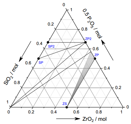
Mason TO, Hummel FA (1974) Compatibility Relations in the System SiO2-ZrO2-P2O5. J Am Ceram Soc 57: 538–539. doi: 10.1111/j.1151-2916.1974.tb10808.x
![]() |
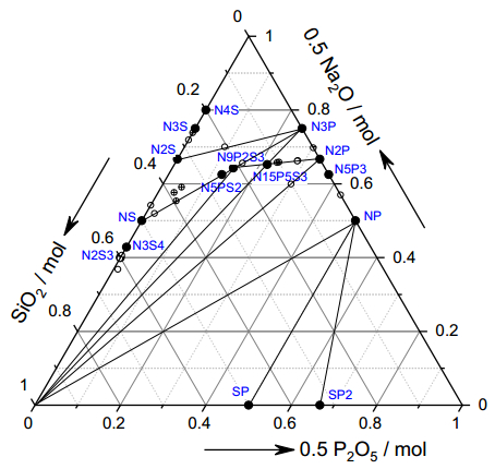
[28] | Turkdogan ET, Maddocks WR (1952) Phase Equilibrium Investigation of the Na2O-SiO2-P2O5 Ternary System. J Iron Steel Inst 172: 1–15. |
[29] | Milne SJ, West AR (1983) Compound formation and conductivity in the system Na2O-ZrO2-P2O5: Sodium zirconium orthophosphates. Solid State Ionics 9–10: 865–868. |
[30] |
Milne SJ, West AR (1985) Zr-Doped Na3PO4: Crystal Chemistry, Phase Relations, and Polymorphism. J Solid State Chem 57: 166–177. doi: 10.1016/S0022-4596(85)80006-2
![]() |
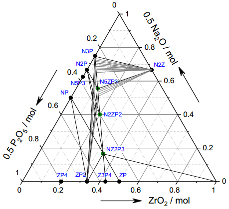
[31] | Vlna M, Petrosyan Y, Kovar V, et al. (1993) Phase Coexistence in the System Na2O-P2O5-ZrO2. Chem Pap 47: 296–297. |
[32] |
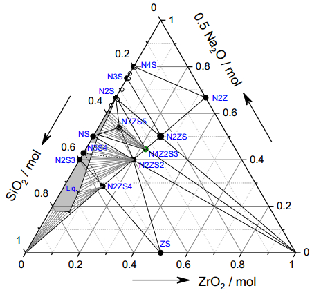
D'Ans J, Löffler J (1930) Untersuchungen im System Na2O-SiO2-ZrO2. Z Anorg Allg Chem 191: 1–35. doi: 10.1002/zaac.19301910102
![]() |
[33] | Polezhaev YM, Chukhlantsev VG (1965) Triangulation of the System Na2O-ZrO2-SiO2. Izv Akad Nauk SSSR Neorg Mater 1: 1990–1993; Inorg Mater (Engl Transl) 1: 1797–1800. |
[34] | Sircar A, Brett NH (1970) Phase Equilibria in Ternary Systems Containing Zirconia and Silica, IV. Preliminary Study of the System Na2O-ZrO2-SiO2. Trans Brit Ceram Soc 69: 131–135. |
[35] | Wilson G, Glasser FP (1987) Subsolidus Phase Relations in the System Na2O-ZrO2-SiO2. Brit Ceram Trans J 86: 199–201. |
[36] |
Nicholas VA, Heyns AM, Kingon AI, et al. (1986) Reactions in the formation of Na3Zr2Si2PO12. J Mater Sci 21: 1967–1973. doi: 10.1007/BF00547935
![]() |
[37] |
Rudolf PR, Subramanian MA, Clearfield A, et al. (1985) The Crystal Structure of a Nonstoichiometric NASICON. Mater Res Bull 20: 643–651. doi: 10.1016/0025-5408(85)90142-4
![]() |
[38] |
Rudolf PR, Clearfield A, Jorgensen JD (1986) Rietveld Refinement Results on Three Nonstoichiometric Monoclinic NASICONs. Solid State Ionics 21: 213–224. doi: 10.1016/0167-2738(86)90075-5
![]() |
[39] |
Yde-Andersen S, Lundgaard JS, Møller L, et al. (1984) Properties of NASICON Electrolytes Prepared from Alkoxide Derived Gels: Ionic Conductivity, Durability in Molten Sodium and Strength Test Data. Solid State Ionics 14: 73–79. doi: 10.1016/0167-2738(84)90014-6
![]() |
[40] |
Perthuis H, Colomban Ph (1986) Sol-Gel Routes Leading to Nasicon Ceramics. Ceram Int 12: 39–52. doi: 10.1016/S0272-8842(86)80008-6
![]() |
[41] | Maier J, Warhus U, Gmelin E (1986) Thermodynamic and Electrochemical Investigations of the NASICON Solid Solution System. Solid State Ionics 18–19: 969–973. |
[42] |
Boilot JP, Collin G, Colomban Ph (1988) Relation Structure-Fast Ion Conduction in the NASICON Solid Solution. J Solid State Chem 73: 160–171. doi: 10.1016/0022-4596(88)90065-5
![]() |
[43] |
Colomban Ph (1986) Orientational Disorder, Glass/Crystal Transition and Superionic Conductivity in NASICON. Solid State Ionics 21: 97–115. doi: 10.1016/0167-2738(86)90201-8
![]() |
[44] |
Park H, Jung K, Nezafati M, et al. (2016) Sodium Ion Diffusion in Nasicon (Na3Zr2Si2PO12) Solid Electrolytes: Effects of Excess Sodium. ACS Appl Mater Interfaces 8: 27814–27824. doi: 10.1021/acsami.6b09992
![]() |
[45] | Kafalas JA, Cava JR (1979) Effect of Pressure and Composition of Fast Na+-Ion Transport in the System Na1+xZr2SixP3−xO12. Proceedings of the International Conference on Fast Ion Transport in Solids, 419–422. |
[46] |
Kreuer KD, Warhus U (1986) NASICON Solid Electrolytes: Part IV Chemical Durability. Mater Res Bull 21: 357–363. doi: 10.1016/0025-5408(86)90193-5
![]() |
1. | Liu Yeling, Wang Jing, 2020, SIR Infectious Disease Model Based on Age Structure and Constant Migration Rate and its Dynamics Properties, 978-1-7281-8571-2, 158, 10.1109/ICPHDS51617.2020.00039 | |
2. | Xiaoguang Li, Xuan Zou, Liming Cai, Yuming Chen, Global dynamics of a vector-borne disease model with direct transmission and differential susceptibility, 2023, 69, 1598-5865, 381, 10.1007/s12190-022-01745-8 | |
3. | Yangyang Shi, Hongyong Zhao, Xuebing Zhang, Threshold dynamics of an age-space structure vector-borne disease model with multiple transmission pathways, 2023, 0, 1534-0392, 0, 10.3934/cpaa.2023035 | |
4. | Meiyu Cao, Jiantao Zhao, Jinliang Wang, Ran Zhang, Dynamical analysis of a reaction–diffusion vector-borne disease model incorporating age-space structure and multiple transmission routes, 2023, 127, 10075704, 107550, 10.1016/j.cnsns.2023.107550 | |
5. | SHUANGSHUANG LIANG, SHENGFU WANG, LIN HU, LIN-FEI NIE, GLOBAL DYNAMICS AND OPTIMAL CONTROL FOR A VECTOR-BORNE EPIDEMIC MODEL WITH MULTI-CLASS-AGE STRUCTURE AND HORIZONTAL TRANSMISSION, 2023, 31, 0218-3390, 375, 10.1142/S0218339023500109 |
ρ | SSTF |
0.03 | FF |
0.04 | dividing point between FF and SF |
0.05 | FF and light SF coexist |
0.25 | FF and heavy SF coexist |
0.45 | SF or FF and SF and Jam coexist(FSJ) |