Research article Special Issues

Characterisation of Ga1-xInxSb quantum wells (x~0.3) grown on GaAs using AlGaSb interface misfit buffer

  • GaInSb multiple quantum wells (MQW) grown on GaAs using an AlGaSb interface misfit (IMF) metamorphic buffer layer technique exhibit superior infrared photoluminescence (PL) at room temperature compared with MQW grown directly on GaSb. PL emission was obtained in the range from 1.7 μm (4 K) to 1.9 μm (300 K) from Ga1-xInxSb samples containing five compressively strained QW with In content x~0.3. Structural and optical characterisation confirms that the AlGaSb IMF growth technique is promising for the development of photonic devices operating at extended wavelengths based on GaAs substrates.

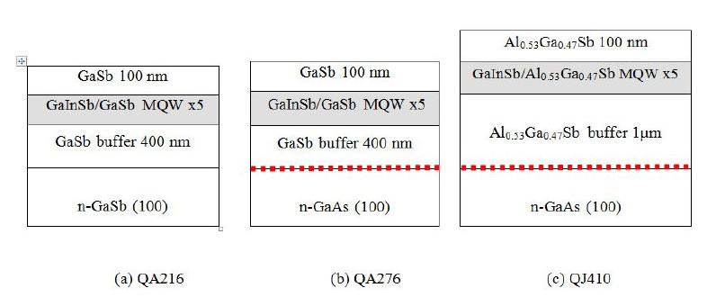
    Citation: Jonathan P. Hayton, Andrew R.J. Marshall, Michael D. Thompson, Anthony Krier. Characterisation of Ga1-xInxSb quantum wells (x~0.3) grown on GaAs using AlGaSb interface misfit buffer[J]. AIMS Materials Science, 2015, 2(2): 86-96. doi: 10.3934/matersci.2015.2.86

    Related Papers:

    [1] Wei Yang, Lili Pan, Jinhui Wan . Smoothing gradient descent algorithm for the composite sparse optimization. AIMS Mathematics, 2024, 9(12): 33401-33422. doi: 10.3934/math.20241594
    [2] Fethi Bouzeffour . Inversion formulas for space-fractional Bessel heat diffusion through Tikhonov regularization. AIMS Mathematics, 2024, 9(8): 20826-20842. doi: 10.3934/math.20241013
    [3] El Mostafa Kalmoun, Fatimah Allami . On the existence and stability of minimizers for generalized Tikhonov functionals with general similarity data. AIMS Mathematics, 2021, 6(3): 2764-2777. doi: 10.3934/math.2021169
    [4] Xuemin Xue, Xiangtuan Xiong, Yuanxiang Zhang . Two fractional regularization methods for identifying the radiogenic source of the Helium production-diffusion equation. AIMS Mathematics, 2021, 6(10): 11425-11448. doi: 10.3934/math.2021662
    [5] Hongwu Zhang, Xiaoju Zhang . Tikhonov-type regularization method for a sideways problem of the time-fractional diffusion equation. AIMS Mathematics, 2021, 6(1): 90-101. doi: 10.3934/math.2021007
    [6] JingJun Yu . Some congruences for $ \ell $-regular partitions with certain restrictions. AIMS Mathematics, 2024, 9(3): 6368-6378. doi: 10.3934/math.2024310
    [7] Phuong Nguyen Duc, Erkan Nane, Omid Nikan, Nguyen Anh Tuan . Approximation of the initial value for damped nonlinear hyperbolic equations with random Gaussian white noise on the measurements. AIMS Mathematics, 2022, 7(7): 12620-12634. doi: 10.3934/math.2022698
    [8] Dun-Gang Li, Fan Yang, Ping Fan, Xiao-Xiao Li, Can-Yun Huang . Landweber iterative regularization method for reconstructing the unknown source of the modified Helmholtz equation. AIMS Mathematics, 2021, 6(9): 10327-10342. doi: 10.3934/math.2021598
    [9] M. J. Huntul, Kh. Khompysh, M. K. Shazyndayeva, M. K. Iqbal . An inverse source problem for a pseudoparabolic equation with memory. AIMS Mathematics, 2024, 9(6): 14186-14212. doi: 10.3934/math.2024689
    [10] Zhenping Li, Xiangtuan Xiong, Jun Li, Jiaqi Hou . A quasi-boundary method for solving an inverse diffraction problem. AIMS Mathematics, 2022, 7(6): 11070-11086. doi: 10.3934/math.2022618
  • GaInSb multiple quantum wells (MQW) grown on GaAs using an AlGaSb interface misfit (IMF) metamorphic buffer layer technique exhibit superior infrared photoluminescence (PL) at room temperature compared with MQW grown directly on GaSb. PL emission was obtained in the range from 1.7 μm (4 K) to 1.9 μm (300 K) from Ga1-xInxSb samples containing five compressively strained QW with In content x~0.3. Structural and optical characterisation confirms that the AlGaSb IMF growth technique is promising for the development of photonic devices operating at extended wavelengths based on GaAs substrates.


    In this paper we consider the problem of finding a stable approximate solution to the ill-posed linear operator equation

    $ Ax=y,
    $
    (1.1)

    where $ A:X: = \ell^2\rightarrow Y $ is a bounded linear operator with non-closed range, i.e., $ \mathrm{range}(A)\neq \overline{\mathrm{range}(A)} $, in the separable Hilbert space $ Y $ with norm $ \|\cdot\| $. We recall that for $ 1\leq p\leq\infty $ the spaces $ \ell^p $ are Banach spaces consisting of (infinite) series $ x = \{x_i\}_{i = 1}^\infty $ with norms $ \|x\|_{\ell^p} = \sqrt[p]{\sum_{i = 1}^\infty |x_i|^p} $ for $ 1\leq p < \infty $ and $ \|\cdot\|_{\ell^\infty} = \sup_{i\in \mathbb{N}}|x_i| $. For $ p = 2 $ one obtains a Hilbert space. We assume that in (1.1) only noisy data $ y^\delta $ is available satisfying the inequality

    $ ||yyδ||δ
    $
    (1.2)

    with known noise level $ \delta > 0 $. In order to determine a stable solution to (1.1) from the noisy data, regularization is required. We are searching for approximations $ x_\alpha^\delta $ of the exact solution $ x^† $ with $ Ax^† = y $ based on the noisy data $ y^\delta $, which are calculated as $ \ell^1 $-regularized solutions

    $ xδα:=argminx2{12||Axyδ||2+α||x||1}
    $
    (1.3)

    with regularization parameters $ \alpha > 0 $. This approach was extensively studied in the last decade and we refer to the brief discussion in Section 4. We remark that the Banach space $ \ell^1 $ is non-reflexive, which makes its analysis challenging. In particular, it was shown in [3,Prop 3.3] that (1.1) is always ill-posed when the domain of $ A $ is restricted to $ \ell^1 $ and $ Y $ is a reflexive Banach space. On the other hand, $ \ell^1 $-regularization in the case $ \|x^†\|_{\ell^1} < \infty $ is well understood as a prominent version of sparsity promoting regularization. Hence, it seems to be of great interest whether the $ \ell^1 $-regularization also makes sense in the oversmoothing case, which is characterized by the fact that $ x^†\in\ell^2\setminus\ell^1 $ such that $ \|x^†\|_{\ell^1} = \infty $. The scenario of oversmoothing regularization has, to the best of the authors knowledge, only been treated in the setting of regularization in Hilbert scales, see Section 2. There, the specific structure of the problem yields link conditions as tools to jump between different scale levels and thus to handle the occurring analytical problems arising from the oversmoothing character of the penalty. For other space settings the corresponding tools are missing, and this paper is an attempt to overcome this deficit. We therefore stress that in this paper we are not interested in specific applications, nor in improving any sort of reconstruction quality. Equation (1.1) and procedure (1.3) merely constitute a new trial case for modeling the oversmoothing regularization.

    Let us now discuss our motivation for investigating this regularization idea. As we will see in our model problem, oversmoothing $ \ell^1 $-regularization already has one advantage over the classical Tikhonov regularization with penalty $ \|\cdot\|_{\ell^2}^2 $, i.e.,

    $ xδα:=argminx2{12||Axyδ||2+α||x||22}.
    $
    (1.4)

    Namely, it does not suffer from the saturation effect of the $ \ell^2 $-regularized approach, and the proposed a priori choice of the regularization parameter coincides with the discrepancy principle for all cases under consideration. Hence, one motivation for oversmoothing regularization are possibly improved convergence properties. But there are more potential benefits. An oversmoothing penalty might yield an easier optimization problem. For example, when $ x^†\in\ell^p\setminus \ell^2 $ with $ p > 2 $, classical Tikhonov regularization (1.4) would be oversmoothing. However, since it is much easier to find the minimizer of the $ \ell^2 $-penalized Tikhonov functional (which corresponds to solving a linear system) than minimizing a functional with arbitrary $ \ell^p $-penalty, the former might be preferred. A third aspect for oversmoothing regularization is feature extraction. In terms of our model problem, $ \ell^1 $-regularization is known to yield sparse regularized solutions, i.e., only finitely many components are non-zero. As we will see later, $ \ell^1 $-regularization in some sense selects the best (least) discretization level to achieve a certain residual. Therefore, the approximate solutions need less storage space than $ \ell^2 $-regularized solutions. In general, other features than sparsity could be of interest. Finally, the analysis of oversmoothing regularization is challenging and might provide new insights for general regularization approaches.

    The paper is organized as follows: In Section 2 we sketch the existing results on oversmoothing regularization in Hilbert scales. We proceed with properties of $ \ell^1 $-regularized solutions and discuss their implications in Section 3. After that we move to convergence rates for $ \ell^1 $-regularization including the oversmoothing case in Section 4. In this context, we restrict our studies to diagonal operators and present a specific simplified model problem, which is the basis for the subsequent numerical experiments. In Section 5 we compare our derived convergence rates with the ones known from classical Tikhonov regularization with $ \ell^2 $-penalty. Finally, numerical experiments supporting the theoretical results are presented in Section 6.

    To the best of the authors knowledge, oversmoothing regularization has so far only been investigated in the setting of regularization in Hilbert scales, starting with the seminal paper by Natterer [6]. There, Natterer considers a linear problem (1.1) between Hilbert spaces X and Y. The regularized solutions are obtained by the minimization problem

    $ xδα:=argminxX{||Axyδ||2+α||x||2p},
    $
    (2.1)

    where the penalty is a norm in a Hilbert scale. In this context, a family $ \{X_s\}_{s\in \mathbb{R}} $ of Hilbert spaces with $ X_0: = X $ is called Hilbert scale if $ X_t\subseteq X_s $ whenever $ s < t $ and the inclusion is a continuous embedding, i.e., there exists $ c_{s, t} > 0 $ such that $ ||x||_s\leq c_{s, t}||x||_t $. The Hilbert scale is induced by an unbounded, self-adjoint, and strictly positive definite operator $ T $ in $ X $ such that $ \|x\|_s: = \|T^s x\|_X $, $ s\in \mathbb{R} $, defines a norm in $ X_s $.

    Under the noise model (1.2) in combination with the smoothness assumption $ ||x^†||_q\leq\rho $ for some $ q > 0 $, and provided that there exists some $ a > 0 $ such that with two constants $ m, M > 0 $ and for all $ x \in X $ the inequality chain

    $ m||x||a||Ax||M||x||a
    $
    (2.2)

    holds true, Natterer shows in [6] the error estimate

    $ xδαxXCδqa+qρaa+q
    $
    (2.3)

    whenever the penalty smoothness $ p $ in (2.1) is sufficiently high, in the sense that $ p \ge (q-a)/2 $, and for the a-priori parameter choice

    $ α(δ)=c(ρ)δ2(a+p)a+q
    $
    (2.4)

    with appropriately chosen constant $ c(\rho) > 0 $. It is interesting that here the index $ p $, which characterizes the smoothness of the penalty in (2.1), is limited for obtaining the rate result (2.3) by a lower bound, but not by an upper bound. Really, Natterer states that ``there is nothing wrong with high order regularization, even well above the order of the smoothness of the exact solution''. Even though $ x^† $ may have arbitrarily small $ q $-norms with $ q > 0 $, one still obtains the order optimal rate of convergence. The only adjustment to be made is an appropriate decrease of the regularization parameter.

    Recently, Natterer's results have been extended to ill-posed inverse problems with nonlinear forward operators by Mathé and Hofmann [7,8]. In the first paper, the regularization parameter is chosen according to the discrepancy principle, while the second paper shows convergence rates under, in principle, the same a-priori parameter choice as occurring in (2.4). In both papers the obtained convergence rate coincides with that in (2.3), i.e., $ \|x_\alpha^\delta-x^†\|_X = \mathcal{O}\left(\delta^\frac{q}{a+q}\right) $ as $ \delta \to 0 $.

    In this section we discuss some basic properties of oversmoothing $ \ell^1 $-regularization or the lack thereof. The results are easily generalized to arbitrary penalty functionals in Tikhonov-type regularization, as long as certain standard assumptions are fulfilled. We refer to, e.g., [9,Assumption 3.11 and Assumption 3.22] or [10,Assumption 8.1] for details. Basic properties of $ \ell^1 $-regularization are well known. As the following lemma shows, existence and stability of regularized solutions with respect to small perturbations in the data are not influenced by the oversmoothing setting.

    Lemma 3.1. For all fixed $ \alpha, \delta > 0 $, a minimizer of (1.3) exists and has a finite $ \ell^1 $-norm. Furthermore, if $ \{y_k\} $ is a sequence norm-converging in $ Y $ to $ y^\delta $, i.e. $ y_k \to y^\delta $, then every associated sequence $ \{x_k\} $ with

    $ x_k\in \mathop {\arg \min }\limits_{x \in \ell^2} \left\{\frac{1}{2}||Ax-y_k||^2+\alpha \|x\|_{\ell^1} \right\} $

    has a subsequence that converges weakly. The weak limit of every such convergent subsequence $ \{x_{\tilde{k}}\} $ of $ \{x_k\} $ is a minimizer $ \tilde{x} $ of (1.3). Moreover, $ \|x_{\tilde{k}}\| $ converges to $ \|\tilde{x}\| $.

    Proof. Take $ \alpha > 0 $ arbitrary but fixed. Since $ \ell^1\subset\ell^2 $, there exists $ \tilde{x}\in \ell^2 $ with finite values $ ||A\tilde x-y^\delta|| $ and $ \|\tilde{x}\|_{\ell^1} $. This implies

    $ \|x_k\|_{\ell^1}\leq \frac{1}{\alpha} \left(\frac{1}{2}\|Ax_k-y_k\|^2+\alpha\|x_k\|_{\ell^1}\right) \leq \frac{1}{\alpha} \left(\frac{1}{2}\|A\tilde x-y_k\|^2+\alpha\|\tilde x\|_{\ell^1}\right) \lt \infty $

    by the optimality of the minimizer. The remaining part of the proof follows from standard arguments [9,10].

    We move on to identify some necessary conditions for the convergence of regularized solutions for $ \delta\rightarrow 0 $ in the case of oversmoothing regularization.

    Theorem 3.1. Let $ x^†\in\ell^2 $ with $ \|x^†\|_{\ell^1} = \infty $ denote a solution to (1.1). If the Tikhonov regularized solutions (1.3) under consideration are weakly convergent to $ x^† $ for an a priori or a posteriori parameter choice rule $ \alpha = \alpha(\delta, y^\delta $), then the following items must hold for a sequence $ x_k: = x_{\alpha_k}^{\delta_k}\rightharpoonup x^† $ as $ \delta_k\rightarrow0 $:

    a) $ \lim_{k\rightarrow\infty}\|x_k\|_{\ell^1} = \infty $,

    b) $ \lim_{k\rightarrow\infty}\alpha_k = 0 $,

    c) $ \lim_{k\rightarrow\infty} \alpha_k\|x_k\|_{\ell^1}\leq C < \infty $.

    Proof. By Lemma 3.1, $ \|x_k\|_{\ell^1} < \infty $ for all $ k\in \mathbb{N} $. If, however, we assume that there is a subsequence $ \{x_{k_j}\} $ with $ \|x_{k_j}\|_{\ell^1}\leq c < \infty $ uniformly for all $ j\in \mathbb{N} $, then the assumed weak convergence $ x_{k_j}\rightharpoonup x^† $ in $ X $ implies that $ \|x^†\|_{\ell^1}\leq c $. This contradicts the assumption $ \|x^†\|_{\ell^1} = \infty $ and yields item a) of the theorem. Now take some fixed $ \tilde x\in\ell^1 $ and keep in mind the definition of the $ x_k $ as minimizers of the functional (1.3). It is

    $ 12||Axkyδk||2+αkxk112||A˜xyδk||2+αk˜x1δ2k+||A˜xy||2+αk˜x1.
    $

    Therefore

    $ \alpha_k(\|x_k\|_{\ell^1}-\|\tilde{x}\|_{\ell^1}) \leq \delta_k^2+||A\tilde{x}-{y}||^2\leq C \lt \infty. $

    Since $ \|\tilde x\|_{\ell^1} < \infty $ we need $ \lim_{k\rightarrow\infty} \alpha_k = 0 $ in order to allow $ \lim_{k\rightarrow \infty} \|x_k\|_{\ell^1} = \infty $ as necessary due to a). Additionally, the product $ \alpha_k\|x_k\|_{\ell^1} $ has to stay bounded, yielding together b) and c).

    The next step would be to show (weak) convergence of the regularized solutions to the exact solution as $ \delta\rightarrow 0 $. However, no such result is known. Even for the Hilbert scale setting of Section 2 no general convergence assertion appears to be available. In the standard setting $ \|x^†\|_{\ell^1} < \infty $, one has due to the optimality of the $ x_\alpha^\delta $

    $ 12Axδαyδ2+αxδα112δ2+αx1<.
    $
    (3.1)

    Requiring $ \alpha\rightarrow 0 $ and $ \delta^2/\alpha\rightarrow 0 $ as $ \delta\rightarrow 0 $ then ensures (weak) convergence of the regularized solutions to the exact one. In particular, the $ \ell^1 $-norm of the regularized solutions $ \| x_\alpha^\delta\|_{\ell^1} $ remains bounded by a constant for all $ \delta > 0 $. In the oversmoothing setting, the right-hand side in (3.1) is infinite, hence provides no useful information. It appears natural to replace $ x^† $ by suitable auxiliary elements to bound the Tikhonov functional, but that is not enough. Let $ \{x_\delta\}_{\delta > 0} $ be a sequence with

    $ \|x_\delta\|_{\ell^1} = \inf\limits_{x\in\ell^2, \|Ax-y\|\leq c\delta}\|x\|_{\ell^1} $

    for fixed constant $ c > 0 $. Using the $ \{x_\delta\}_{\delta > 0} $ to bound the Tikhonov functional, we obtain

    $ 12Axδαyδ2+αxδα112Axδyδ2+αxδ1(c+1)δ2+αxδ1.
    $
    (3.2)

    For any choice of $ \alpha = \alpha(\delta) $ one obtains $ \| x_\alpha^\delta\|_{\ell^1}\leq c\frac{\delta^2}{\alpha}+\|x_\delta\|_{\ell^1} $. Even if $ \delta^2/\alpha\rightarrow 0 $, this does not yield a bound for $ \| x_\alpha^\delta\|_{\ell^1} $ independent of $ \delta $, since $ \|x_\delta\|_{\ell^1}\rightarrow \infty $. Therefore one cannot infer the existence of a (weakly) convergent subsequence among the regularized solutions $ x_\alpha^\delta $ as is the argument in the standard, non-oversmoothing, convergence results. For the oversmoothing regularization one would need that the $ x_\alpha^\delta $ are bounded in a norm weaker than the $ \ell^1 $-norm, for example, in the $ \ell^2 $-norm. It is currently not clear how such a connection can be established. At this point we also mention that the oversmoothing approach prevents the use of state-of-the-art regularization theory. In recent years, variational inequalities (sometimes also called variational source conditions) have emerged as a powerful tool in the theory of Banach-space regularization, and we only refer, for example, to the papers [4,5]. For $ \ell^1 $ regularization, in [11] a variational inequality of the form

    $ xx1x1x1+φ(AxAx)
    $
    (3.3)

    for a well-defined concave index function $ \varphi $ and valid for all $ x \in \ell^1 $ was established and used for deriving convergence rates in the case $ x^† \in \ell^1 $. Clearly, this concept is inapplicable when $ x^† \in \ell^2 \setminus \ell^1 $ and hence $ \|x^†\|_{\ell^1} = \infty $, but it could be an idea to measure the error in $ \ell^2 $-norms. Therefore, it seems to be interesting that not even for $ x^† \in \ell^1 $ a variational inequality of the form

    $ \|x-x^†\|^\kappa_{\ell^2}\leq \|x\|_{\ell^1}-\|x^†\|_{\ell^1}+\varphi(\|Ax-Ax^†\|) $

    with $ \kappa = 1 $ or $ \kappa = 2 $ is known as an alternative to (3.3).

    In this section, we derive convergence rates for the $ \ell^1 $-penalized Tikhonov-type regularization (1.3) to (1.1). This method became a popular and powerful tool in the last decade, sparked by the seminal paper [13]. Since then, many authors have contributed to its theory and application. Here we only mention the papers [14,15,16]. As is typical in $ \ell^1 $-regularization, we assume that $ A $ is injective. For the non-injective case we refer to [17]. The vast majority of papers connected to $ \ell^1 $-regularization assumes sparsity in the sense that $ x^†\in\ell^0 $, i.e., that it has only finitely many non-zero components. However, in [11] for the first time the situation that the exact solution $ x^† $ is not sparse, but only $ x^†\in\ell^1 $, was explored. The results were later refined and extended in [3,12,18,19]. In some sense, this paper is a continuation of this development as we are now interested in the case that $ x^† $ is not even in $ \ell^1 $, but $ x^†\in\ell^2\setminus \ell^1 $. Due to this we will employ the $ \ell^2 $-norm to measure the speed of convergence, and we seek for an index function $ \varphi $, i.e., a continuous, monotonically increasing, and concave function with $ \varphi(0) = 0 $, such that

    $ ||x_\alpha^\delta-x^†||_{\ell^2}\leq C\varphi(\delta) $

    holds with some constant $ C > 0 $. We will show that an appropriate choice of the regularization parameter yields such a function $ \varphi $.

    It is well-known that $ \ell^1 $-regularization yields sparse solutions. We will see that for showing convergence rates when $ x^†\notin \ell^1 $ it is essential to estimate the support of the regularized solutions. In order to do this, we rely on the explicit calculation of the minimizers. Therefore, we have to restrict ourselves to diagonal operators for this paper. We denote by $ \{e^{(i)}\}_{i = 1}^\infty $ the canonical orthonormal basis in $ \ell^2 $ with components $ e^{(k)}_k = 1 $ and $ e^{(i)}_k = 0 $ for $ k\not = i $. Moreover, we denote by $ \{v^{(i)}\}_{i = 1}^\infty $ an orthonormal basis in the range closure $ \overline{\mathrm{range}(A)} $ of $ Y $. Then we say that a compact operator $ A: \ell^2 \to Y $ with decreasingly ordered singular values $ \{\sigma_i\}_{i = 1}^\infty $ is of diagonal structure if

    $ A e^{(i)} = \sigma_i v^{(i)} \quad \mbox{and} \quad e^{(i)} = \frac{1}{\sigma_i} A^*v^{(i)} \quad (i = 1, 2, ...). $

    This model includes compact linear operators mapping between general Hilbert spaces $ X $ and $ Y $, since such operators can be diagonalized with respect to their singular system [1,2].

    We now present a way of constructing functions $ \varphi $ that serve as prototypes for convergence rates. To this end, we define, for all $ n\in \mathbb{N} $, the linear projectors

    $ Pn:22,Pnx={xi}ni=1.
    $
    (4.1)

    Lemma 4.1. Let $ A:\ell^2 \to Y $ be a compact linear operator with diagonal structure as introduced above, possessing the singular values

    $ \|A\| = \sigma_1 \ge \sigma_2 \ge ... \ge \sigma_n \ge \sigma_{n+1} \ge ... \to 0 \qquad \mathit{\mbox{as}} \quad n \to \infty, $

    and let $ x^†\in\ell^2 $ denote the uniquely determined solution to the operator equation (1.1), and set

    $ T(x,n):=||(IPn)x||2=i=n+1|xi|2.
    $
    (4.2)

    Then for any $ x\in\ell^2 $ it is, for all $ n\in \mathbb{N} $,

    $ ||xx||2||(IPn)x||2+σ1n||AxAx||+T(x,n).
    $
    (4.3)

    Proof. We have, for any $ x\in\ell^2 $, with the linear projectors from (4.1) the relation

    $ ||xx||2||(IPn)x||2+||Pn(xx)||2+||(IPn)x||2
    $
    (4.4)

    which holds for all $ n\in \mathbb{N} $. We keep $ n $ arbitrary but fixed and start estimating the last term which describes the decay of the tail of the solution and thus its smoothness. It is a fixed function of $ n $ which goes to zero as $ n\rightarrow \infty $, and we employ the convention (4.2).

    Next we estimate the middle term $ ||P_n(x-x^†)||_{\ell^2} $ in (4.4). In order to do so we recall the notion of the modulus of continuity, given by

    $ ω(M,θ):=sup{||x||:xM,||Ax||θ}
    $

    where $ M\subset \ell^2 $. This quantity is essentially related to minimal errors of any regularization method for noisy data. Since $ P_n(x-x^†)\in \ell^2_n: = \rm{span}\{e_1, \dots, e_n\} $, we can use tools from approximation theory to estimate its norm. In [20,Proposition 3.9] it has been shown that for any finite dimensional space $ X_n $

    $ \omega(X_n, \theta) = \frac{\theta}{\Theta(A, n)}, $

    where the modulus of injectivity $ \Theta(A, n) $ is defined as

    $ \Theta(A, n): = \inf\limits_{0\neq x\in X_n} \frac{||Ax||}{||x||}. $

    For diagonal operators it is $ \Theta(A, n) = \sigma_n $ and thus

    $ ω(2n,θ)=σ1nθ.
    $

    Noting that for diagonal operators it also holds that

    $ ||APn(xx)||||A(xx)||,
    $
    (4.5)

    it is therefore

    $ ||Pn(xx)||2ω(2n,||APn(xx)||)=σ1n||APn(xx)||σ1n||A(xx)||.
    $
    (4.6)

    Inserting this and (4.2) into (4.4), we obtain (4.3).

    In the best case scenario the term $ ||(I-P_n)x||_{\ell^2} $ in (4.3) vanishes (note that this is a crucial point to be shown for the $ \ell^1 $-regularized approximations to $ x^† $) and only the two rightmost terms remain. The best possible convergence rate is therefore determined by taking the infimum of those two expressions with respect to $ n $. This yields a prototype rate function

    $ φ(t)=infnN{tσn+(IPn)x2}.
    $
    (4.7)

    Note that as infimum over affine functions $ \varphi $ is concave, and it is also monotonically increasing with $ \varphi(0) = 0 $. Since for fixed $ t\geq 0 $ the infimum is taken over a countable set and $ \sigma_n^{-1} t\rightarrow\infty $ monotonically as $ n\rightarrow\infty $ while $ \mathcal{T}(x^†, n)\rightarrow 0 $ monotonically, the infimum is attained as minimum and the corresponding index

    $ ninf(t):=argminnN{tσn+(IPn)x2}
    $
    (4.8)

    is well defined. In order to show $ ||x-x^†||_{\ell^2}\leq \varphi(\|Ax-Ax^†\|) $ for the $ \ell^1 $-regularized solutions $ x = x_\alpha^\delta $ from (1.3), we need the following assumptions.

    Assumption 4.1. (a) The singular values of $ A $ fulfill, for all $ n\in \mathbb{N} $,

    $ 1\leq\frac{\sigma_n}{\sigma_{n+1}}\leq C_\sigma $

    with a constant $ 1\leq C_\sigma < \infty $.

    (b) The tail is monotone, i.e., $ |x_n^†| $ is monotonically decreasing for all sufficiently large $ n $.

    (c) The convergence rate $ \varphi(t) $ is not dominated by the tail, i.e., there exists a constant $ \tilde C $ such that

    $ \mathcal{T}(x^†, n_{\mathrm{inf}}(t))\leq \tilde C \sigma_{ n_{\mathrm{inf}}(t)}^{-1}t. $

    (d) For the true solution $ x^† $ it holds

    $ |x_{ n_{\mathrm{inf}}(t)+1}^†|\leq \mathcal{C} \frac{\sigma_{ n_{\mathrm{inf}}(t)}^{-1}t}{\sqrt{n_{ n_{\mathrm{inf}}(t)}}} $

    for a constant $ 0\leq \mathcal{C} < \infty $ and sufficiently small $ t > 0 $.

    Part (a) limits the ill-posedness of the forward operators. A polynomial decay of the singular values fulfills the condition, even an exponential decay of order $ \sigma_i = e^{-i} $ is permitted, but for any $ {ilon}_{\varepsilon} > 0 $ a decay $ \sigma_i = e^{-i^{1+{ilon}_{\varepsilon}}} $ violates the condition. Note that the left-hand inequality is trivial, but will be used in a proof later. Part (b) is required purely for technical reasons. Part (c) and (d) link the smoothness of the true solution with the ill-posedness of the forward operator. They will be discussed in examples below. We remark that similar restrictions are standing assumptions in the Hilbert-scale setting of Section 2: Condition (2.2) ensures that the singular values of $ A $ fall asymptotically as $ i^{-a} $, and the condition $ p\geq (q-a)/2 $ implies that the solution must not be significantly smoother than the penalty.

    For later use we mention two consequences of Assumption 4.1.

    Lemma 4.2. Let $ A $ be as in Lemma 4.1, and let Assumption 4.1 (a) and (c) hold. Then

    $ 11+˜Cφ(t)σ1ninf(t)tφ(t).
    $
    (4.9)

    Furthermore, it is

    $ APninf(t)xAx˜Ct.
    $
    (4.10)

    Proof. The right-hand inequality of (4.9) follows from the definition of $ \varphi $ in (4.7). Similarly, it is

    $ \varphi(t) = \sigma_{ n_{\mathrm{inf}}(t)}^{-1}t+\mathcal{T}(x^†, n_{\mathrm{inf}}(t))\leq (1+\tilde C)\sigma_{ n_{\mathrm{inf}}(t)}^{-1}t, $

    which yields the left-hand inequality. To obtain the estimate of the residual, we observe that

    $ APninf(t)xAx2=i=ninf(t)+1|σixi|2σ2ninf(t)+1i=ninf(t)+1|xi|2σ2ninf(t)T(x,ninf(t))2.
    $

    Inserting Assumption 4.1 (c) immediately yields (4.10).

    In order to show convergence rates based on Lemma 4.1, two terms need to be estimated in (4.3) for $ x = x_\alpha^\delta $: the residual $ \|Ax_\alpha-Ax^†\| $ and the tail $ \|(I-P_n) x_\alpha^\delta\|_{\ell^2} $.

    Lemma 4.3. Let $ A $ be as in Lemma 4.1, and let Assumption 4.1 (c) hold. Then, with the a-priori choice

    $ α(δ)=cαδ2ninf(δ)φ(δ),
    $
    (4.11)

    with constant $ 0 < c_\alpha < \infty $, the minimizers $ x_\alpha^\delta $ of (1.3) satisfy

    $ ||Axδαyδ||((˜C+1)2+4cα)δ.
    $
    (4.12)

    In particular, it is

    $ AxδαAxcδ
    $
    (4.13)

    with positive constant $ c = (\tilde C+1)^2+4c_\alpha+1 $.

    Proof. From the Tikhonov functional (1.3) we have for all $ n\in \mathbb{N} $

    $ 12||Axδαyδ||2+α||xδα||112||APnxyδ||2+α||Pnx||1,
    $

    which with

    $ ||x_\alpha^\delta||_{\ell^1} = ||P_nx_\alpha^\delta||_{\ell^1}+||(I-P_n)x_\alpha^\delta||_{\ell^1} $

    and

    $ ||P_nx^†||_{\ell^1}\leq ||P_n(x^†-x_\alpha^\delta)||_{\ell^1}+||P_n x_\alpha^\delta||_{\ell^1} $

    yields

    $ 12||Axδαyδ||2+α||(IPn)xδα||112||APnxyδ||2+α||Pn(xxδα)||112APnxyδ2+αnPn(xxδα)2.
    $
    (4.14)

    Now fix $ n = n_{\mathrm{inf}}(\delta) $. Using (4.6) and (4.9) on the right-hand side we have

    $ ||Pninf(δ)(xxδα)||2σ1ninf(δ)AxδαAxσ1ninf(δ)(Axδαyδ+Axyδ)2σ1ninf(δ)max{Axδαyδ,δ}2φ(Axδαyδ),
    $
    (4.15)

    where in the last estimate we have assumed $ \|A x_\alpha^\delta-y^\delta\| > \delta $, as otherwise the assertion of the lemma is trivially fulfilled. We combine this estimate with (4.14) and again set $ n = n_{\mathrm{inf}}(\delta) $. This yields

    $ 12||Axδαyδ||212||APninf(δ)xyδ||2+2αninf(δ)φ(||Axδαyδ)||).
    $
    (4.16)

    Note that by (4.10) we have $ ||AP_{ n_{\mathrm{inf}}(\delta)}x^†-y^\delta||\leq (\tilde C+1) \delta $. Inserting the parameter choice (4.11) into (4.16), we continue analogously to [5,Corollary 1]. Namely, it is by concavity of $ \varphi $

    $ 12||Axδαyδ||2(˜C+1)22δ2+2cαδ2ninf(δ)φ(δ)ninf(δ)φ(||Axδαyδ)(˜C+1)22δ2+2cαδ2φ(Axδαyδ)φ(δ)δ2((˜C+1)22+2cα)φ(Axδαyδ)φ(δ)δ2((˜C+1)22+2cα)Axδαyδφ(δ)δφ(δ)=δ((˜C+1)22+2cα)Axδαyδ.
    $

    This yields $ ||Ax_\alpha^\delta-y^\delta||\leq ((\tilde C+1)^2+4 c_\alpha)\delta $ for $ \alpha $ from (4.11).

    The second assertion follows from this, the noise assumption (1.2), and the triangle inequality.

    Lemma 4.4. Let $ A $ be as in Lemma 4.1, and let Assumption 4.1 (a)–(d) hold. Let $ \alpha $ be chosen according to (4.11) such that $ c_\alpha\geq \mathcal{C}(\tilde C+1) $. Then the minimizers $ x_\alpha^\delta $ of (1.3) satisfy

    $ (IPninf(δ))xδα)2Cσφ(δ).
    $
    (4.17)

    Proof. The diagonal structure of the operator allows to calculate the minimizer of (1.3) explicitly, and (1.3) reads

    $ 12||Axyδ||2+α||x||1=12iN(σixiyδi)2+αiN|xi|.
    $
    (4.18)

    Since the components are decoupled, the first order optimality condition for the above functional is

    $ \frac{\partial}{\partial x_i}\left(\frac{1}{2}\sum\limits_{i\in \mathbb{N}}(\sigma_ix_i-y^\delta_i)^2+\alpha\sum\limits_{i\in \mathbb{N}}|x_i|\right) = 0\quad \forall i\in \mathbb{N}, $

    i.e., for each $ i\in \mathbb{N} $,

    $ \sigma_i(\sigma_ix_i-y^\delta_i)+\alpha \mathrm{sgn}(x_i) = 0 $

    where

    $ \mathrm{sgn}(x): = {1x>01x<0[1,1]x=0
    . $

    Consider the case $ [x_\alpha^\delta]_i > 0 $. Then

    $ [x_\alpha^\delta]_i = \frac{y^\delta_i}{\sigma_i}-\frac{\alpha}{\sigma_i^2} \gt 0. $

    On the other hand, for $ [x_\alpha^\delta]_i < 0 $ we have

    $ [x_\alpha^\delta]_i = \frac{y^\delta_i}{\sigma_i}+\frac{\alpha}{\sigma_i^2} \lt 0 $

    and consequently

    $ [xδα]i=0|yδiσi|ασ2i.
    $
    (4.19)

    We will only consider the case $ [x_\alpha^\delta]_i > 0 $ further, the results for $ [x_\alpha^\delta]_i < 0 $ are analogous with inverted sign. First let $ y $ be exact, noise-free data, i.e., $ y_i = \sigma_ix_i^† $ for all $ i\in \mathbb{N} $, where the minimizer of (4.18) (with $ y^\delta $ temporarily replaced by $ y $) is denoted by $ x_\alpha $. Then (4.19) yields

    $ [xα]i=0|xi|ασ2i.
    $
    (4.20)

    Inserting the parameter choice (4.11) and considering $ i = n_{\mathrm{inf}}(\delta)+1 $, we find with Assumption 4.1 (a) and (d), and with (4.9) that

    $ ασ2ninf(δ)+1=ασ2ninf(δ)σ2ninf(δ)σ2ninf(δ)+1cα(σ1ninf(δ)δ)2ninf(δ)φ(δ)cα˜C+1σ1ninf(δ)δninf(δ)cαC(˜C+1)|xninf(δ)+1|.
    $

    Now, as long as $ c_\alpha\geq \mathcal{C}(\tilde C+1) $, this implies $ [x_\alpha]_{ n_{\mathrm{inf}}(\delta)+1} = 0 $. Because $ \frac{\alpha}{\sigma_{i}^2} $ is increasing in $ i $ while $ |x^†_i| $ decreases, we conclude that for $ n_{\mathrm{inf}}(\delta) $ sufficiently large (i.e., $ \delta $ sufficiently small), $ [x_\alpha]_{ n_{\mathrm{inf}}+1} = 0 $. Under Assumption 4.1 (b) all entries $ [x_\alpha]_{m} $, $ m > n_{\mathrm{inf}}(\delta) $, must then also be zero. Hence, in the noise-free case, we have $ \|(I-P_{ n_{\mathrm{inf}}(\delta)})x_\alpha\|_{\ell^2} = 0 $. Therefore, for noisy data and under the same parameter choice, any contribution to $ \|(I-P_{ n_{\mathrm{inf}}(\delta)}) x_\alpha^\delta\|_{\ell^2} $ must be due to the noise in the data. Consider the model $ y-y^\delta = \delta\zeta $ with some $ \zeta\in\ell^2 $, $ ||\zeta||_{\ell^2} = 1 $. Then $ \|y-y^\delta\| = \delta $ and

    $ [xδα]i>0xi+δζiσiασ2i>0.
    $
    (4.21)

    The components $ x_i^† $ are fixed and decreasing. The regularization parameter $ \alpha $ is fixed for all $ i $, hence $ \alpha/\sigma_i^2 $ grows with increasing index. Therefore, the smaller $ i $, the (potentially) larger the components $ [x_\alpha^\delta]_i $ could become. To estimate the tail $ ||(I-P_{ n_{\mathrm{inf}}(\delta)})x_\alpha^\delta||_{\ell^2} $ we are only interested in the higher indices $ i > n_{\mathrm{inf}}(\delta) $. Due to the asymptotics of the individual terms, $ ||(I-P_{ n_{\mathrm{inf}}(\delta)})x_\alpha^\delta||_{\ell^2} $ therefore becomes largest when all its mass is concentrated in the lowest possible component $ n_{\mathrm{inf}}(\delta)+1 $, i.e., $ \zeta_{ n_{\mathrm{inf}}(\delta)+1} = 1 $ and $ (I-P_{ n_{\mathrm{inf}}(\delta)})x_\alpha^\delta = ([x_\alpha^\delta]_{ n_{\mathrm{inf}}(\delta)+1}, 0, \dots) $. From the noise-free considerations above we already obtained $ x_i^†\leq \frac{\alpha}{\sigma_i^2} $. Hence, any positive contribution in (4.21) comes from the noise. With an analogous argument for the case $ [x_\alpha^\delta]_i < 0 $ we therefore get

    $ |[x_\alpha^\delta]_{ n_{\mathrm{inf}}(\delta)+1}|\leq \frac{\delta}{\sigma_{ n_{\mathrm{inf}}(\delta)+1}}. $

    Using Assumption 4.1 (c) we obtain

    $ \frac{\delta}{\sigma_{ n_{\mathrm{inf}}(\delta)+1}} = \frac{\delta}{\sigma_{ n_{\mathrm{inf}}(\delta)}}\frac{\sigma_{ n_{\mathrm{inf}}(\delta)}}{\sigma_{ n_{\mathrm{inf}}(\delta)+1}}\leq C_\sigma \sigma_{ n_{\mathrm{inf}}(\delta)}^{-1}\delta\leq C_\sigma\varphi(\delta). $

    Putting all the pieces together yields the main theorem.

    Theorem 4.1. Let $ A:\ell^2 \to Y $ be a compact linear operator with diagonal structure, possessing the singular values

    $ \|A\| = \sigma_1 \ge \sigma_2 \ge ... \ge \sigma_n \ge \sigma_{n+1} \ge ... \to 0 \qquad \mathit{\mbox{as}} \quad n \to \infty. $

    Let $ x^†\in\ell^2 $ denote the uniquely determined solution to the operator equation (1.1), and let Assumption 4.1 hold. Then the $ \ell^1 $-regularized solutions $ x_\alpha^\delta $ from (1.3) with noisy data $ y^\delta $ obeying the noise model $ \|y-y^\delta\|\leq\delta $ satisfy for sufficiently small $ \delta > 0 $ the estimate

    $ ||xδαx||2(Cσ+c)φ(δ)
    $

    with $ c $ as in (4.13) and with the concave index function

    $ φ(t)=infnN{tσn+(IPn)x2},
    $

    provided the regularization parameter is chosen a priori as

    $ α(δ)=cαδ2ninf(δ)φ(δ),
    $

    with constant $ c_\alpha\geq \mathcal{C}(\tilde C+1) $. The integers

    $ ninf(δ):=argminnN{δσn+(IPn)x2}
    $

    can be found for all $ \delta > 0 $.

    Proof. Lemma 4.1 and the discussion thereafter provide us with the prototype of the convergence rate $ \varphi(t) $ (4.7) and with $ n_{\mathrm{inf}}(t) $ (4.8). Consider (4.3) with $ x $ replaced by $ x_\alpha^\delta $, i.e.,

    $ ||xδαx||2||(IPn)xδα||2+σ1n||AxδαAx||+T(x,n).
    $
    (4.22)

    Fix $ n = n_{\mathrm{inf}}(\delta) $. From Lemma 4.3 we then have $ \|A x_\alpha^\delta-Ax^†\|\leq c \delta $ with $ c > 1 $, hence

    $ || x_\alpha^\delta-x^†||_{\ell^2}\leq ||(I-P_{ n_{\mathrm{inf}}(\delta)}) x_\alpha^\delta||_{\ell^2}+ c(\sigma_{ n_{\mathrm{inf}}(\delta)}^{-1} \delta+ \mathcal{T}(x^†, n_{\mathrm{inf}}(\delta))). $

    The term in brackets, by definition, attains the value $ \varphi(\delta) $. The remaining term $ ||(I-P_{ n_{\mathrm{inf}}(\delta)}) x_\alpha^\delta||_{\ell^2} $ was estimated in Lemma 4.4. Therefore

    $ \| x_\alpha^\delta-x^†\|_{\ell^2}\leq (C_\sigma+c)\varphi(\delta). $

    The a-priori choice requires, in principle, the knowledge of the exact solution and is thus unfeasible in practice. In the following we comment on the discrepancy principle as an a-posteriori parameter choice. We begin with a helpful lemma.

    Lemma 4.5. Let Assumption 4.1 hold and $ \alpha_\ast(\delta) $ be any choice of the regularization parameter in (1.3) such that

    $ \tau_1\delta\leq \|Ax_{\alpha_\ast}^\delta-y^\delta\|\leq \tau_2\delta $

    for $ (1+\tilde C) < \tau_1\leq\tau_2 < \infty $. Then $ \bar c\alpha_\ast\geq \alpha $ with the a-priori choice of $ \alpha $ from (4.11) and $ \bar c = \frac{2c_\alpha(\tau_2+1)}{\tau_1^2-(\tilde C+1)^2} $.

    Proof. From the minimizing property of the Tikhonov-functional we have

    $ \frac{1}{2}\|Ax_{\alpha_\ast}^\delta-y^\delta\|^2+\alpha_\ast\|x_{\alpha_\ast}^\delta\|_{\ell^1}\leq \frac{1}{2}\|AP_{ n_{\mathrm{inf}}(\delta)}x^†-y^\delta\|^2+\alpha_\ast\|P_{ n_{\mathrm{inf}}(\delta)}x^†\|_{\ell^1}. $

    Similar to the proof of Lemma 4.3 this implies

    $ 12||Axδαyδ||212||APninf(δ)xyδ||2+αninf(δ)φ(||AxδαAx)||).
    $
    (4.23)

    Note that for this results we have replaced (4.15) by

    $ ||P_{ n_{\mathrm{inf}}(\delta)}(x^†-x_\alpha^\delta)||_{\ell^2}\leq \sigma_{ n_{\mathrm{inf}}(\delta)}^{-1}\|A x_\alpha^\delta-Ax^†\|\leq \varphi(\|A x_\alpha^\delta-Ax^†\|). $

    Using $ ||AP_{ n_{\mathrm{inf}}(\delta)}x^†-y^\delta||\leq (\tilde C+1) \delta $ (cf. Lemma 4.2) and $ \tau_1\delta\leq \|Ax_{\alpha_\ast}^\delta-y^\delta\| $ in (4.23) we have

    $ \frac{\tau_1^2\delta^2}{2}\leq \frac{(\tilde C+1)^2}{2}\delta^2+\alpha_\ast\sqrt{ n_{\mathrm{inf}}(\delta)} \varphi(||Ax_\alpha^\delta-Ax^†)||), $

    and since $ \tau_1 > (1+\tilde C) $

    $ \delta^2\leq \frac{2}{\tau_1^2-(\tilde C+1)^2}\alpha_\ast\sqrt{ n_{\mathrm{inf}}(\delta)} \varphi(||Ax_\alpha^\delta-Ax^†)||). $

    Using the upper bound $ \|Ax_{\alpha_\ast}^\delta-y^\delta\|\leq \tau_2\delta $ and the concavity of $ \varphi $, it is

    $ \varphi(||Ax_\alpha^\delta-Ax^†||)\leq \varphi(||Ax_\alpha^\delta-y^\delta||+||y^\delta-Ax^†||)\leq (\tau_2+1)\varphi(\delta) $

    and we obtain, with $ \alpha $ from (4.11),

    $ \alpha = c_\alpha\frac{\delta^2}{\sqrt{ n_{\mathrm{inf}}(\delta)}\varphi(\delta)}\leq c_\alpha \frac{2(\tau_2+1)}{\tau_1^2-(\tilde C+1)^2}\alpha_\ast. $

    Theorem 4.2. Let $ A:\ell^2 \to Y $ be a compact linear operator with diagonal structure, possessing the singular values

    $ \|A\| = \sigma_1 \ge \sigma_2 \ge ... \ge \sigma_n \ge \sigma_{n+1} \ge ... \to 0 \qquad \mathit{\mbox{as}} \quad n \to \infty. $

    Let $ x^†\in\ell^2 $ denote the uniquely determined solution to the operator equation (1.1), and let Assumption 4.1 hold. Then the $ \ell^1 $-regularized solutions $ x_\alpha^\delta $ from (1.3) with noisy data $ y^\delta $ obeying the noise model $ \|y-y^\delta\|\leq\delta $ satisfy for sufficiently small $ \delta > 0 $ the estimate

    $ ||xδαx||2(τ2+Cσ+1)φ(δ)
    $

    with a constant $ 0 < c < \infty $ and with the concave index function

    $ φ(t)=infnN{tσn+(IPn)x2},
    $

    provided the regularization parameter is chosen a posteriori such that

    $ τ1δAxδαyδτ2δ,
    $
    (4.24)

    with parameters $ 1+\tilde C < \tau_1\leq\tau_2 < \infty $ such that $ \frac{2\mathcal{C}(\tilde C +1)(\tau_2+1)}{\tau_1^2-(\tilde C+1)^2}\leq 1 $.

    Proof. We start as in the proof of Theorem 4.1 and consider (4.22). Due to the parameter choice (4.24) and the triangle inequality we have

    $ \|A x_\alpha^\delta-Ax^†\|\leq (\tau_2+1)\delta, $

    hence it is, with $ n = n_{\mathrm{inf}}(\delta) $,

    $ || x_\alpha^\delta-x^†||_{\ell^2}\leq ||(I-P_{ n_{\mathrm{inf}}(\delta)}) x_\alpha^\delta||_{\ell^2}+ (\tau_2+1)(\sigma_{ n_{\mathrm{inf}}(\delta)}^{-1} \delta+ \mathcal{T}(x^†, n_{\mathrm{inf}}(\delta))) = ||(I-P_{ n_{\mathrm{inf}}(\delta)}) x_\alpha^\delta||_{\ell^2}+ (\tau_2+1)\varphi(\delta). $

    According to Lemma 4.3, the regularization parameter $ \alpha_\ast $ obtained from the discrepancy principle is larger than the a-priori parameter $ a $ from (4.11), $ \alpha\leq \alpha_\ast $, if $ \bar c\leq 1 $. The minimal admissible constant $ c_\alpha $ in Lemma 4.4 is $ c_\alpha = \mathcal{C}(\tilde C+1) $. Inserting this into $ \bar c $ yields $ \alpha\leq\alpha_\ast $ if $ \frac{2\mathcal{C}(\tilde C +1)(\tau_2+1)}{\tau_1^2-(\tilde C+1)^2}\leq 1 $. It now follows analogously as in the proof of Lemma 4.4 that for noise-free data $ ||(I-P_{ n_{\mathrm{inf}}(\delta)}) x_\alpha^\delta||_{\ell^2} = 0 $ and in the worst-case noise scenario $ ||(I-P_{ n_{\mathrm{inf}}(\delta)}) x_\alpha^\delta||_{\ell^2}\leq C_\sigma\varphi(\delta) $. Hence

    $ || x_\alpha^\delta-x^†||_{\ell^2}\leq (\tau_2+C_\sigma+1)\varphi(\delta). $

    In order to exemplify and illustrate the general theory in more detail, we will now consider some simple model scenarios. As before, we assume that $ A:\ell^2\rightarrow\ell^2 $ is diagonal, $ [Ax]_i = \sigma_ix_i $, $ i = 1, 2, \dots $. For simplicity, we will denote all constants by a generic constant $ 0 < c < \infty $.

    Let $ \sigma_i = i^{-\beta} $ and $ x^†_i = i^{-\eta} $ for positive values $ \beta $ and $ \eta $ and all $ i\in \mathbb{N} $. In particular, for $ \frac{1}{2} < \eta\leq 1 $ this yields a case of oversmoothing regularization $ \|x^†\|_{\ell^1} = \infty $, whereas for $ \eta > 1 $ we have the classical model with $ \|x^†\|_{\ell^1} < \infty $.

    Theorem 4.3. Let $ A $ be diagonal with singular values $ \sigma_i = i^{-\beta} $, $ \beta > 0 $. Let $ x^†\in\ell^2 $ be such that $ [x^†]_i = i^{-\eta} $ for $ \eta > \frac{1}{2} $. Then the $ \ell^1 $-regularized solutions $ x_\alpha^\delta $ from (1.3) to (1.1), with noisy data $ y^\delta $ obeying $ \|y-y^\delta\|\leq\delta $, satisfy

    $ ||xδαx||2cδ2η12η+2β1,
    $
    (4.25)

    provided the regularization parameter is chosen a priori as

    $ α(δ)=cδ4β+2η2η+2β1
    $
    (4.26)

    or according to the discrepancy principle (4.24).

    Proof. It remains to calculate the quantities occurring in the proof of Theorem 4.1 explicitly.

    The tail of the exact solution satisfies

    $ ||(IPn)x||2=i=n+1|iη|212η1(n+1)12η(2η1)12n12η.
    $
    (4.27)

    Inserting the structure of $ A $, the rate prototype (4.7) becomes

    $ φ(t)=infnN{nβt+cηn12η}.
    $
    (4.28)

    It is simple calculus to show

    $ φ(t)=ct2η12η+2β1
    $

    and

    $ ninf(t)=ct22η+2β1
    $
    (4.29)

    where $ \lceil\cdot\rceil $ denotes the closest integer. Inserting the previous results into the parameter choice (4.11) yields

    $ α(δ)=δ2ninf(δ)φ(δ)=cδ4β+2η2η+2β1.
    $
    (4.30)

    We mention that this model problem fulfills Assumption 4.1. Namely, we have $ x_{n+1} < x_n = n^{-\eta} $ for all $ n\in \mathbb{N} $, and from (4.27) we obtain

    $ \frac{\|(I-P_{n})x^†\|_{\ell^2}}{\sqrt{n}}\leq c n^{-\eta}. $

    Also Assumption 4.1 (c) is fulfilled as

    $ 1\leq\frac{\sigma_n}{\sigma_{n+1}}\leq \frac{n^{-\beta}}{(n+1)^{-\beta}} = \left(\frac{n+1}{n}\right)^\beta\leq2^\beta = :C_\sigma. $

    Finally, we observe that

    $ \frac{\delta^2}{\alpha} = \frac{\delta^2}{c\delta^{\frac{4\beta+2\eta}{2\eta+2\beta-1}}} = c\delta^{\frac{2\eta-2}{2\eta+2\beta-1}} $

    goes to infinity when $ \frac{1}{2} < \eta < 1 $, stays constant for $ \eta = 1 $, and goes to zero for $ \eta > 1 $. That means there is a seamless transition between the regime of oversmoothing regularization and that of classical regularization. Numerical experiments are presented in Section 6.

    We now consider for simplicity the case $ \sigma_i = i^{-1} $ and $ x_i^† = e^{-i} $ for all $ i\in \mathbb{N} $. This is no oversmoothing regularization since $ x^†\in\ell^1 $. Using MATHEMATICA®we calculate the tail in (4.7), $ \mathcal{T}(x^†, n)\leq ce^{-n} $. It is then simple calculus to show

    $ n_{inf}(t) = c\ln\frac{1}{t}. $

    This yields

    $ \varphi(t) = \sigma_{ n_{\mathrm{inf}}(t)}^{-1}t+ \mathcal{T}(x^†, n_{\mathrm{inf}}(t)) = c( t\ln\frac{1}{t}+t). $

    In contrast to the previous example, the two terms $ \sigma_{ n_{\mathrm{inf}}(\delta)}^{-1}\delta $ and $ \mathcal{T}(x^†, n_{\mathrm{inf}}(\delta)) $ are no longer of the same order, but, for sufficiently small $ \delta $, $ \sigma_{ n_{\mathrm{inf}}(\delta)}^{-1}\delta $ is the dominating part, i.e., Assumption 4.1 (c) is fulfilled. Also part (d) of Assumption 4.1 holds, since $ x_{ n_{\mathrm{inf}}(\delta)+1}^† < x_{ n_{\mathrm{inf}}(\delta)}^† = c\delta $, whereas $ \frac{\sigma_{ n_{\mathrm{inf}}(\delta)}^{-1}\delta}{\sqrt{ n_{\mathrm{inf}}(\delta)}} = c\delta\sqrt{\ln(\frac{1}{\delta})} $. The predicted rate $ \| x_\alpha^\delta-x^†\|_{\ell^2}\leq c\varphi(\delta) = c\delta\ln\frac{1}{\delta} $ can be verified numerically, see the left plot of Figure 5.

    Figure 5.  Numerically observed convergence rate for model cases 4.3.2 (left) and the sparsity case 4.3.5 (right) where Assumption 4.1 holds. In both cases we have a good fit between measured and theoretical convergence rate. Note that in the sparsity case, only the first 4 components of $ x^† $ were non-zero. The regularized approximation $ x_\alpha^\delta $ had at most 5 non-zero entries.

    Let now $ \sigma_i = e^{-i} $ and, for simplicity, $ x^†_i = i^{-1} $ for all $ i\in \mathbb{N} $. We are again in the oversmoothing regime. To formulate the convergence rate, we recall the definition of the Lambert-W-function, defined as $ z = W(ze^z) $. With this, the minimizing argument of

    $ \varphi(t) = \inf\limits_{n\in \mathbb{N}} e^nt+cn^{-\frac{1}{2}} $

    can be found, using MATHEMATICA®, to be

    $ n_{\mathrm{inf}}(t) = \left\lceil \frac{3}{2}W\left(\frac{2}{3}t^{-\frac{3}{2}}\right) \right\rceil, $

    such that

    $ \varphi(t) = te^{ n_{\mathrm{inf}}(t)}+c n_{\mathrm{inf}}(t)^{-\frac{1}{2}}. $

    The first term decays faster than the second one, hence the rate is dominated by the tail of the exact solution, and Assumption 4.1 (c) is violated, see Figure 1. Consequently, Theorem 4.1 is not applicable. Indeed, in a numerical experiment, shown in the left part of Figure 6, the measured convergence rate is different from the one predicted here.

    Figure 1.  $ \delta e^{ n_{\mathrm{inf}}(\delta)} $ (red, dashed), $ n_{\mathrm{inf}}(\delta)^{-\frac{1}{2}} $ (black, solid), and $ \varphi(\delta) $ (blue, dash-dotted), for the scenario of Section 4.3.3, demonstrating the violation of Assumption 4.1 (c).
    Figure 6.  Numerically observed convergence rate for the model cases 4.3.3 (left) and 4.3.4 (right) where Assumption 4.1 is violated. In the left-hand plot, predicted and measured convergence rate show a clear mismatch, indicating that Assumption 4.1 is indeed needed for our analysis. On the right-hand side we see a good match between theoretical and measured rates. We attribute this to the phenomenon discussed in Section 4.3.4, namely that Assumption 4.1 (d) does not hold for all $ \delta > 0 $, but for all numerically reasonable $ \delta > \delta_0 > 0 $.

    Let for this example $ \sigma_i = e^{-i} $ and $ x_i^† = e^{-i} $ for all $ i\in \mathbb{N} $. Then

    $ \varphi(t) = \inf\limits_{n\in \mathbb{N}} e^nt+ce^{-n} $

    and

    $ n_{\mathrm{inf}}(t) = \frac{1}{2}\ln\left(\frac{1}{t}\right), $

    hence

    $ \varphi(t) = c(e^{\frac{1}{2}\ln(\frac{1}{t})}t+e^{-\frac{1}{2}\ln(\frac{1}{t})}) = c\sqrt{t}. $

    Because $ x_{ n_{\mathrm{inf}}(\delta)+1}^† < x_{ n_{\mathrm{inf}}(\delta)}^† = c\sqrt{\delta} $, but $ \frac{\sigma_{ n_{\mathrm{inf}}(\delta)}^{-1}\delta}{\sqrt{ n_{\mathrm{inf}}(\delta)}} = c\sqrt{\frac{\delta}{\ln(\frac{1}{\delta})}} $, Assumption 4.1 (d) is (formally) violated. Numerically, however, even for values of $ \delta $ significantly smaller then the machine-$ {ilon}_{\varepsilon} $, a constant can be found such that Assumption 4.1 (d) holds, i.e., $ \sqrt{\delta}\leq \mathcal{C}(\delta_0) \sqrt{\frac{\delta}{\ln(\frac{1}{\delta})}} $ for $ \delta > \delta_0 $. A plot exemplifying this can be found in Figure 2. Consequently, our numerically retrieved convergence rate is close to the predicted $ \sqrt{\delta} $-rate, see the right part of Figure 6.

    Figure 2.  Scenario of Section 4.3.4: In general, this example violates Assumption 4.1 (d), but for $ \delta > 10^{-30} $, the assumption is valid with $ \mathcal{C} = 10 $.

    Our last examples goes back to the setting that sparked the developments around $ \ell^1 $-regularization, namely the case of sparse solutions. Let $ x^† = (x_1^†, x_2^†, \dots, x_{n_0}^†, 0, 0, \dots) $. Let $ A $ be as in Theorem 4.1 with no further restrictions. Then

    $ \varphi(t) = \inf\limits_{n\in \mathbb{N}} \sigma_n^{-1}t+\sum\limits_{i = n+1}^{\infty}|x_i^†| = \min\left\lbrace \inf\limits_{n\in \mathbb{N}, n\leq n_0} \sigma_n^{-1}t+\sum\limits_{i = n+1}^{n_0}|x_i^†|, \sigma_{n_0+1}^{-1}t \right\rbrace, $

    i.e., (only) for sufficiently small values of $ \delta $ can a linear convergence rate $ \varphi(\delta) = c\delta $ be reached. Note that in the literature the linear convergence rate was derived in the $ \ell^1 $-norm, $ \| x_\alpha^\delta-x^†\|_{\ell^1}\leq c\delta $, whereas we obtain the same rate in the $ \ell^2 $-norm $ \| x_\alpha^\delta-x^†\|_{\ell^2}\leq c\delta $. Since for sufficiently small $ \delta > 0 $ $ n_{\mathrm{inf}}(\delta) = n_0+1 = \mathrm{const} $, we also recover from (4.11) the well-known parameter choice $ \alpha = c\delta $.

    In order to get a feeling for the derived convergence rate we compare the result from the previous section with classical, non-oversmoothing, $ \ell^1 $-regularization and $ \ell^2 $-regularization. In order to be able to use explicit expressions for the convergence rates and parameter choice rules, we will only consider the specific model problem of Section 4.3.1. Let us start with classical $ \ell^1 $-regularization, i.e., the approximate solution to (1.1) is obtained via (1.3) but under the assumption that $ ||x^†||_{\ell^1} < \infty $. In [19] a convergence rate

    $ ||x_\alpha^\delta-x^†||_{\ell^1}\leq c\delta^{\frac{\eta-1}{\eta+\beta-\frac{1}{2}}} = :\varphi_{\ell^1}(\delta) $

    was derived using the parameter choice

    $ \alpha(\delta) \sim\frac{\delta^2}{\varphi_{\ell^1}(\delta)} = c\delta^{\frac{4\beta+2\eta}{2\eta+2\beta-1}}. $

    Now let us move to $ \ell^2 $-regularization. This corresponds to the classic Tikhonov regularization, i.e., the approximate solution to (1.1) is given by (1.4). It is then well known, see e.g. [1,2], that under the assumption

    $ xrange((AA)ν)
    $
    (5.1)

    for some $ 0\leq\nu\leq 2 $ the best possible convergence rate

    $ ||xδαx||2cδνν+1
    $
    (5.2)

    can be shown under the a-priori parameter choice

    $ \alpha(\delta)\sim\delta^{\frac{2}{\nu+1}}. $

    In the diagonal setting of Section 4.3 the source condition (5.1) can easily be related to the parameters $ \eta $ and $ \beta $. Namely, (5.1) holds for all $ \nu $ with $ \frac{2\eta-1}{2\beta} > \nu $ [21]. Since we are interested in the largest $ \nu $ we set $ \nu = \frac{2\eta-1}{2\beta} $ for simplicity, acknowledging that actually we should write $ \nu = \frac{2\eta-1}{2\beta}+{ilon}_{\varepsilon} $ for arbitrary but small $ {ilon}_{\varepsilon} > 0 $. With this, the convergence rate becomes

    $ ||x_\alpha^\delta-x^†||_{\ell^2}\leq c\delta^{\frac{\nu}{\nu+1}} = c\delta^\frac{2\eta-1}{2\eta+2\beta-1} = \varphi(\delta) $

    with $ \varphi(\delta) $ from (4.25), and the parameter choice is

    $ \alpha(\delta)\sim\frac{\delta^2}{\varphi(\delta)^2} = \frac{\delta^2}{\delta^{\frac{4\eta-2}{2\eta+2\beta-1}}} = \delta^{\frac{4\beta}{2\eta+2\beta-1}}. $

    We summarize the convergence rates and parameter choices in Table 1. One sees that the $ \ell^1-\ell^2 $-regularization, corresponding to $ \ell^1 $-regularization with the $ \ell^2 $-norm as error measure which includes the oversmoothing regularization, inherits the parameter choice from the classical $ \ell^1 $-regularization and the convergence rate from the classical $ \ell^2 $-regularization. The parameter choice influences the residual $ ||Ax_\alpha^\delta-y^\delta|| $ and the penalty value $ ||x_\alpha^\delta||_{\ell^1} $. Since it is most important to keep the residual on a level of about $ \delta $, the $ \ell^1 $-parameter choice is used. This is in line with [18] where it has been observed that for $ \ell^1 $-regularization the regularization parameter obtained via discrepancy principle and a-priori parameter choice always coincide up to constant factors. It is however somewhat surprising that this property appears to remain even when $ x^†\notin\ell^1 $. The less smooth the solution is, the smaller $ \alpha $ has to be chosen. On the other hand, the optimal convergence rate in $ \ell^2 $ is well known to be given by (5.2). Therefore $ \ell^1 $-regularization yields the optimal ($ \ell^2 $-)convergence rate, even when $ x^†\notin\ell^1 $. Even more, it does not saturate like classical $ \ell^2 $ regularization which possesses the qualification $ \nu = \frac{2\eta-1}{2\beta}\leq 2 $. Take any $ \frac{1}{2} < \eta\leq 1 $. Then $ x^†\in \ell^2\backslash \ell^1 $. If $ \beta < \frac{\eta}{2}-\frac{1}{4} $, then $ \nu > 2 $ and $ \ell^2 $-regularization (1.4) has saturated with the limiting convergence rate $ \varphi(\delta)\sim\delta^{2/3} $. Oversmoothing $ \ell^1 $-regularization, on the other hand, would yield a higher rate of convergence since it does not saturate.

    Table 1.  Comparison of (classical) $ \ell^1 $, (classical) $ \ell^2 $ and (oversmoothing) $ \ell^1-\ell^2 $ regularization for the diagonal setting of Section 4.1. The parameter choice depends on the penalty functional whereas the convergence rate depends on the norm the regularization error is measured in.
    Type $ \ell^1 $ $ \ell^1-\ell^2 $ $ \ell^2 $
    rate $ \varphi_{\ell^1}(\delta)=\delta^{\frac{2\eta-2}{2\eta+2\beta-2}} $ $ \varphi_{\ell^2}(\delta)=c\delta^\frac{2\eta-1}{2\eta+2\beta-1} $ $ \varphi_{\ell^2}(\delta)=c\delta^\frac{2\eta-1}{2\eta+2\beta-1} $
    $ \alpha $ $ \delta^{\frac{4\beta+2\eta}{2\eta+2\beta-1}} $ $ \delta^{\frac{4\beta+2\eta}{2\eta+2\beta-1}} $ $ \delta^{\frac{4\beta}{2\eta+2\beta-1}} $
    $ \alpha $ recipe $ \alpha=\frac{\delta^2}{\varphi_{\ell^1}} $ $ \alpha=\frac{\delta^2}{\varphi_{\ell^2}(\delta)\delta^{\frac{-1}{2\eta+2\beta-1}}} $ $ \alpha=\frac{\delta^2}{\varphi_{\ell^2}(\delta)} $

     | Show Table
    DownLoad: CSV

    In this section we consider an operator specifically tailored to the setting of Section 4.1. We start with the Voltera operator

    $ [˜Ax](s)=s0x(t)dt
    $

    and discretize $ \tilde A $ with the rectangular rule at $ N = 400 $ points. In order to ensure our desired properties of the model cases of Section 4.3 we compute the SVD of the resulting matrix and manually set its singular values $ \sigma_i $ accordingly. This means that the actual operator $ A $ in (1.1) is an operator possessing the same singular vectors $ \{u_i\} $ and $ \{v_i\} $ as $ \tilde A $, but different singular values $ \{\sigma_i\} $. Using the SVD, we construct our solution such that $ x_i^† = \langle x^†, v_i\rangle $ holds according to the scenario. We add random noise to the data $ y = Ax^† $ such that $ ||y-y^\delta|| = \delta $. The range of $ \delta $ is such that the relative error is between $ 25\% $ and $ 0.2\% $. The solutions are computed via

    $ x_\alpha^\delta = \text{argmin} \left\lbrace||Ax-y^\delta||^2+\alpha ||x||_{\ell_1}\right\rbrace, $

    where the $ \ell^1 $-norm is taken using the coefficients with respect to the basis originating from the SVD. We compute the reconstruction error in the $ \ell_2 $ norm as well as the residuals. For larger values of $ \eta $ we can observe the convergence rate directly. For smaller values of $ \eta $, we have to compensate for the error introduced by the discretization level. Namely, since we use a discretization level $ N = 400 $, numerically we actually measure

    $ ||P_{400}(x_\alpha^\delta-x^†)||_{\ell^2} $

    with the projectors $ P $ as before being the cut-off after $ N = 400 $ elements. In the plots of the convergence rates we show

    $ ||P400(xδαx)+(IP400)x||2.
    $
    (6.1)

    The second term can be calculated analytically and is supposed to correct for the fact that we cannot measure the regularization error for coefficients corresponding to larger $ n $, i.e., we add the tail of $ x^† $ that can not be observed. Because $ x_\alpha^\delta $ has only finitely many non-zero components and we use a sufficiently large discretization, we do not make any error with respect to the tail of the solutions.

    Our main focus is on the fully diagonal case of Section 4.3.1, i.e, $ \sigma_i = i^{-\beta} $ for $ \beta > 0 $ and $ x_i^† = i^{-\eta} $ for $ \eta > \frac{1}{2} $. Here, the regularization parameter is chosen a-priori according to (4.26) with $ c_\alpha = 1 $.

    We show selected plots of the convergence rates in Figure 3 for $ \beta = 1 $ and Figure 4 for $ \beta = 2 $. The plots are given with logarithmic scales for both axis. In each plot of the convergence rates we added the regression line for the assumption $ ||x_\alpha^\delta-x^†||_{\ell^2} = c \delta^e $. The value of $ e $ is given in the legend. The regularization parameter is shown in the title of the figures in the form $ \alpha = \delta^a $, $ a $ given. The result of our simulations for a larger number of parameters $ \eta $ are shown in Tables 2 and 3 for $ \beta = 1 $ and $ \beta = 2 $, respectively. We see that for all values of $ \eta $ the predicted and measured convergence rate coincides nicely. Additionally, the residual remains stable around $ ||Ax_\alpha^\delta-y^\delta||\sim\delta $. For small values of $ \eta $ and $ \beta = 1 $ the residual is a bit smaller than expected. We suppose this is due to the cut-off of $ x^† $ due to the discretization. For correct results we would have to include a tail of the residual similar to (6.1). If $ \eta $ is very large, i.e. the components of the solution decay rapidly, the observed convergence rate is basically linear. We suppose this is due to numerical effects as numerically those solutions are de facto sparse.

    Figure 3.  Numerically observed convergence rates for $ \beta = 1 $ and $ \eta\in\{0.55, 0.7\} $. From the measured reconstruction error (solid line) we calculated the regression for the assumption $ ||x_\alpha^\delta-x^†||_{\ell^2} = c \delta^e $, shown in the broken line. The theoretical convergence rate (4.25) is matched almost perfectly.
    Figure 4.  Numerically observed convergence rates for $ \beta = 2 $ and $ \eta\in\{0.55, 1.05\} $. From the measured reconstruction error (solid line) we calculated the regression for the assumption $ ||x_\alpha^\delta-x^†||_{\ell^2} = c \delta^e $, shown in the broken line. The theoretical convergence rate (4.25) is matched almost perfectly.
    Table 2.  Convergence rates for $ \beta = 1 $ and various values $ \eta $. $ \alpha $ in the form $ \alpha = \delta^a $. Measured and predicted regularization error in the form $ ||x_\alpha^\delta-x^†||_{\ell^2} = c \delta^e $. Residual given in the form $ ||Ax_\alpha^\delta-y^\delta|| = c \delta^d $.
    $ \eta $ $ \alpha $, $ a $ measured rate, $ e $ predicted rate, $ e $ residual, $ d $
    0.55 2.42 0.047 0.048 1.1
    0.6 2.36 0.09 0.091 1.08
    0.7 2.25 0.163 0.166 1.06
    0.8 2.15 0.229 0.23 1.028
    0.9 2.07 0.284 0.286 1.007
    1 2 0.33 0.333 1.01
    1.05 1.97 0.359 0.355 1.006
    1.1 1.94 0.372 0.375 1.006
    1.3 1.83 0.458 0.444 1.01
    1.5 1.75 0.515 0.5 1.01
    2 1.6 0.595 0.6 1.01
    2.5 1.5 0.659 0.667 0.996
    3 1.42 0.698 0.714 0.996
    6 1.23 0.81 0.85 0.997

     | Show Table
    DownLoad: CSV
    Table 3.  Convergence rates for $ \beta = 2 $ and various values $ \eta $. $ \alpha $ in the form $ \alpha = \delta^a $. Measured and predicted regularization error in the form $ ||x_\alpha^\delta-x^†||_{\ell^2} = c \delta^e $. Residual given in the form $ ||Ax_\alpha^\delta-y^\delta|| = c \delta^d $.
    $ \eta $ $ \alpha=\delta^a $, $ a $ measured rate, $ e $ predicted rate, $ e $ residual, $ d $
    0.55 2.22 0.024 0.024 1.0005
    0.6 2.19 0.0473 0.0476 1.002
    0.7 2.13 0.089 0.091 1.01
    0.8 2.09 0.128 0.13 1.006
    0.9 2.04 0.166 0.167 1.006
    1.01 1.996 0.209 0.203 0.999
    1.1 1.96 0.236 0.23 0.994
    1.3 1.89 0.284 0.286 1.002
    1.5 1.83 0.329 0.333 0.999
    1.75 1.76 0.384 0.385 0.996
    2 1.71 0.421 0.428 0.999

     | Show Table
    DownLoad: CSV

    Finally, we compare the theoretically predicted convergence rates from the remaining model cases of Section 4.3 to measured rates from numerical experiments. In all experiments, the regularization parameter was chosen according to the discrepancy principle (4.24) with $ \tau_1 = 1.1 $ and $ \tau_2 = 1.3 $. We obtained a good match between the theoretical and observed convergence rates in the cases of sections 4.3.2, 4.3.4, and 4.3.4. Only case 4.3.3 showed a significant difference. This is no surprise, since Assumption 4.1 does not hold in this case.

    We have shown that oversmoothing regularization, i.e., Tikhonov regularization with a penalty that takes the value infinity in the exact solution, yields existence and stability of regularized solutions. We have discussed why it is difficult to show convergence of regularized solutions to the true solution in the limit of vanishing data noise. For the specific case of Tikhonov-regularization with $ \ell^1 $-penalty term under a diagonal operator we have derived convergence rates of regularized solutions to the true solution even if those does not belong to $ \ell^1 $ anymore. The theoretical convergence rates have been verified numerically for a model problem.

    D. Gerth was funded by Deutsche Forschungsgemeinschaft (DFG), project HO1454/10-1.

    The authors declare there is no conflicts of interest in this paper.

    [1] Pascal-Delannoy F, Bouganot J, Allogho G, et al. (1992) MOVPE grown Ga0.6In0.4Sb photodiodes for 2.55um detection. Electron Lett 28: 531-532.
    [2] Bertru N, Baranov A, Cuminal Y, et al. (1998) Long-wavelength (Ga, In)Sb/GaSb strained quantum well lasers grown by molecular beam epitaxy. Semicond Sci Technol 13: 936. doi: 10.1088/0268-1242/13/8/019
    [3] Krier A, Sherstnev V (2000) Powerful interface light emitting diodes for methane gas detection. J Phys D Appl Phys 33: 101. doi: 10.1088/0022-3727/33/2/301
    [4] Refaat T, Abedin M, Koch G, et al. (2003) Infrared detector characterization for CO2 DIAL measurement. in Proc. SPIE 5154, Lidar Remote Sensing for Environmental Monitoring IV, San Diego, California, USA.
    [5] Rotter TJ, Tatebayashi J, Senanayake P, et al. (2009) Continuous-Wave, Room-Temperature Operation of 2-μm Sb-Based Optically-Pumped Vertical-External-Cavity Surface-Emitting Laser Monolithically Grown on GaAs Substrates. Appl Phys Express 2: 112102. doi: 10.1143/APEX.2.112102
    [6] Demeo D, Shemelya C, Downs C, et al. (2014) GaSb Thermophotovoltaic Cells Grown on GaAs Substrate Using the Interfacial Misfit Array Method. J Electronic Mater 43: 902-908. doi: 10.1007/s11664-014-3029-1
    [7] Craig A, Marshall A, Tian Z, et al. (2013) Mid-infrared InAs0.79Sb0.21-based nBn photodetectors with Al0.9Ga0.2As0.1Sb0.9 barrier layers, and comparisons with InAs0.87Sb0.13 p-i-n diodes, both grown on GaAs using interfacial misfit arrays. Appl Phys Lett 103: 253502.
    [8] Huang S, Balakrishnan G, Huffaker D (2009) Interfacial misfit array formation for GaSb growth on GaAs. J Appl Phys 105: 103104. doi: 10.1063/1.3129562
    [9] Reyner C, Wang J, Nunna K, et al. (2011) Characterization of GaSb/GaAs interfacial misfit arrays using x-ray diffraction. Appl Phys Lett 99: 231906. doi: 10.1063/1.3666234
    [10] Akahane K, Yamamoto N, Gozu S, et al. (2006) (In)GaSb/AlGaSb quantum wells grown on Si substrates. Thin Solid Films 515: 4467-4470.
    [11] Jin S, Sweeney S (2003) High-Pressure Studies of Recombination Mechanisms in 1.3um GaInNAs Quantum-Well Lasers. IEEE J Sel Top Quantum Electron 9: 1196. doi: 10.1109/JSTQE.2003.819515
  • This article has been cited by:

    1. Daniel Gerth, Bernd Hofmann, Christopher Hofmann, 2020, Chapter 9, 978-981-15-1591-0, 177, 10.1007/978-981-15-1592-7_9
    2. Philip Miller, Thorsten Hohage, Maximal spaces for approximation rates in 1
    -regularization, 2021, 149, 0029-599X, 341, 10.1007/s00211-021-01225-4
    3. De-Han Chen, Bernd Hofmann, Irwin Yousept, Oversmoothing Tikhonov regularization in Banach spaces * , 2021, 37, 0266-5611, 085007, 10.1088/1361-6420/abcea0
  • Reader Comments
  • © 2015 the Author(s), licensee AIMS Press. This is an open access article distributed under the terms of the Creative Commons Attribution License (http://creativecommons.org/licenses/by/4.0)
通讯作者: 陈斌, bchen63@163.com
  • 1. 

    沈阳化工大学材料科学与工程学院 沈阳 110142

  1. 本站搜索
  2. 百度学术搜索
  3. 万方数据库搜索
  4. CNKI搜索

Metrics

Article views(5910) PDF downloads(983) Cited by(1)

/

DownLoad:  Full-Size Img  PowerPoint
Return
Return

Catalog