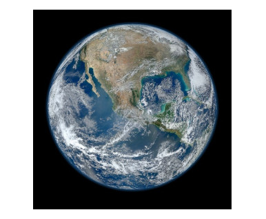
This paper examines our understanding of climate change, as well as the reluctance of industrial societies to deal with the drivers, especially the burning of the fossil fuels, before the future consequences become catastrophic. We describe how the energy balance of the Earth, oceans, land and Arctic sea ice are maintained, and how climate is warming and changing with increases in the three most important greenhouse gases: carbon dioxide from burning fossil fuels, water vapor from evaporation off a warmer ocean, and methane from several sources. We discuss the Earth's water cycle and the role of evaporation, latent heat and condensation in driving storms, transporting energy poleward and giving increasing precipitation extremes, floods, droughts and fires. We review the increasing challenge of meeting human demand for water as water tables are falling globally from increased pumping, and winter snowpack storage is shrinking. We discuss rising sea level, the challenges of long-term carbon storage and the lessons from the past four ice age cycles. The text is written for scientific and public audiences, both global and in the US, so metric and US units are given. The social, moral and ethical choices are mapped by contrasting the Earth-centered indigenous worldview needed for our survival with the industrial mindset that is willing to destroy a stable climate to keep the profits of the current economy growing. We review the long history of the misuse of human power, the rise of science and technology without a guiding moral framework, and how neoliberal capitalism by default makes choices that are driving rapid climate change. We outline how deceit by the matrix of corporations and fossil fuel interests that we call the Fossil Empire has prevented government regulation for decades and accelerated the climate crisis.
Citation: Alan K Betts. Climate change and society[J]. AIMS Geosciences, 2021, 7(2): 194-218. doi: 10.3934/geosci.2021012
This paper examines our understanding of climate change, as well as the reluctance of industrial societies to deal with the drivers, especially the burning of the fossil fuels, before the future consequences become catastrophic. We describe how the energy balance of the Earth, oceans, land and Arctic sea ice are maintained, and how climate is warming and changing with increases in the three most important greenhouse gases: carbon dioxide from burning fossil fuels, water vapor from evaporation off a warmer ocean, and methane from several sources. We discuss the Earth's water cycle and the role of evaporation, latent heat and condensation in driving storms, transporting energy poleward and giving increasing precipitation extremes, floods, droughts and fires. We review the increasing challenge of meeting human demand for water as water tables are falling globally from increased pumping, and winter snowpack storage is shrinking. We discuss rising sea level, the challenges of long-term carbon storage and the lessons from the past four ice age cycles. The text is written for scientific and public audiences, both global and in the US, so metric and US units are given. The social, moral and ethical choices are mapped by contrasting the Earth-centered indigenous worldview needed for our survival with the industrial mindset that is willing to destroy a stable climate to keep the profits of the current economy growing. We review the long history of the misuse of human power, the rise of science and technology without a guiding moral framework, and how neoliberal capitalism by default makes choices that are driving rapid climate change. We outline how deceit by the matrix of corporations and fossil fuel interests that we call the Fossil Empire has prevented government regulation for decades and accelerated the climate crisis.

| [1] | Betts AK (1976) Letter to the Editor on "Scientists in Society". Bull Amer Meteorol Soc 57: 460. Available from: https://alanbetts.com/research/paper/letter-to-the-editor-on-scientists-in-society/#abstract. |
| [2] | UNFCCC (1992) Available from: https://en.wikipedia.org/wiki/United_Nations_Framework_Convention_on_Climate_Change. |
| [3] | Blue River Declaration (2011) Available from: https://liberalarts.oregonstate.edu/sites/liberalarts.oregonstate.edu/files/blue_river_declaraton.dec.2011_.pdf. |
| [4] | Mann ME (2021) The New Climate War: the fight to take back our planet. Public Affairs, New York. |
| [5] |
Mann ME, Bradley RS, Hughes MK (1999) Northern hemisphere temperatures during the past millennium: Inferences, uncertainties, and limitations Geophys Res Lett 26: 759-762. doi: 10.1029/1999GL900070

|
| [6] | Watson RT, Albritton DL, Barker T, et al. (2001) Climate Change 2001, Summary for Policy Makers, IPCC Third Assessment Report. Available from: https://www.ipcc.ch/site/assets/uploads/2018/03/spm.pdf. |
| [7] |
Betts AK, Desjardins R, Worth D (2016) The Impact of Clouds, Land use and Snow Cover on Climate in the Canadian Prairies. Adv Sci Res 13: 37-42. doi: 10.5194/asr-13-37-2016
|
| [8] |
Kwok R, Rothrock DA (2009) Decline in Arctic sea ice thickness from submarine and ICESat records: 1958-2008. Geophys Res Lett 36: 5. doi: 10.1029/2009GL039035
|
| [9] |
Hansen J, Nazarenko L (2004) Soot climate forcing via snow and ice albedos. Proc Natl Acad Sci USA 101: 423-428. doi: 10.1073/pnas.2237157100
|
| [10] | Myhre G, Shindell D, Bréon FM, et al. (2013) Anthropogenic and Natural Radiative Forcing. Climate Change 2013: The Physical Science Basis. Contribution of Working Group I to the Fifth Assessment Report of the Intergovernmental Panel on Climate Change. Cambridge University Press, Cambridge, United Kingdom and New York, NY, USA. |
| [11] |
Lacis AA, Schmidt GA, Rind D, et al (2010) Atmospheric CO2: Principal Control Knob Governing Earth's Temperature. Science 330: 356-359. doi: 10.1126/science.1190653
|
| [12] | Keeling CD, Bacastow RB, Bainbridge AE, et al. (1976) Atmospheric carbon dioxide variations at Mauna Loa Observatory, Hawaii. Tellus 28: 538-551. |
| [13] |
Karion A, Sweeney C, Pétron G, et al. (2013) Methane emissions estimate from airborne measurements over a western United States natural gas field. Geophy Res Lett 40: 1-5. doi: 10.1002/grl.50811
|
| [14] |
Johnson MR, Tyner DR, Conley S, et al. (2017) Comparison of airborne measurements and inventory estimates of methane emissions in the Alberta upstream oil and gas sector. Environ Sci Technol 51: 13008-13017. doi: 10.1021/acs.est.7b03525
|
| [15] | Cai Y, Cai XH, Desjardins RL, et al. (2020) Methane emissions from a waste treatment site: Numerical analysis of aircraft-based data. Agric For Meteorol 292-293. |
| [16] | Dyer J, Desjardins R (2020) Protein as a Unifying Metric for Carbon Footprinting Livestock. Available from: https://researchoutreach.org/wp-content/uploads/2020/10/James-Dyer-and-Raymond-Desjardins.pdf. |
| [17] |
Hansen J, Sato M, Kharecha P, et al. (2008) Target Atmospheric CO2: Where Should Humanity Aim? Open Atmos Sci J 2: 217-231. doi: 10.2174/1874282300802010217
|
| [18] |
Betts AK, Ridgway W (1989) Climatic equilibrium of the atmospheric convective boundary layer over a tropical ocean. J Atmos Sci 46: 2621-2641. doi: 10.1175/1520-0469(1989)046<2621:CEOTAC>2.0.CO;2
|
| [19] | Betts AK, Betts H (2017) From Inside the Eye of the Storm: Hurricane Irma. Rutland Herald. Available from: https://alanbetts.com/writings/articles/from-inside-the-eye-of-the-storm-hurricane-irma/. |
| [20] | Betts AK (2017) Surviving Maria in Puerto Rico. Rutland Herald. Available from: https://alanbetts.com/writings/articles/surviving-maria-in-puerto-rico/. |
| [21] | IPCC (2007) Regional Climate Projections. AR4-WG1. Available from: http://www.ipcc.ch/publications_and_data/ar4/wg1/en/ch11.html. |
| [22] |
Francis JA, Vavrus SJ, Cohen J (2017) Amplified Arctic warming and mid-latitude weather: new perspectives on emerging connections. WIREs Clim Change 8: e474. doi: 10.1002/wcc.474
|
| [23] | Hayhoe K. Kossin J, Kunkel K, et al. (2014) NCA4 report, Figure 2.18. Available from: https://nca2014.globalchange.gov/report/our-changing-climate/heavy-downpours-increasing. |
| [24] |
Guilbert J, Betts AK, Rizzo DM, et al. (2015) Characterization of increased persistence and intensity of precipitation in the Northeastern United States. Geophys Res Lett 42: 1888-1893. doi: 10.1002/2015GL063124
|
| [25] | Betts AK (2012) Climate change: Taking a Local Perspective to the Global Level. Earthzine. Available from: https://earthzine.org/climate-change-taking-a-local-perspective-to-the-global-level/. |
| [26] |
Famiglietti JS (2014) The global groundwater crisis. Nature Clim Change 4: 945-948. doi: 10.1038/nclimate2425
|
| [27] |
Nicholls RJ, Lincke D, Hinkel J, et al. (2021) A global analysis of subsidence, relative sea level change and coastal flood exposure. Nature Clim Change 11: 338-342. doi: 10.1038/s41558-021-00993-z
|
| [28] | Madani N, Parazoo NC, Kimball JS, et al. (2020) Recent Amplified Global Gross Primary Productivity Due to Temperature Increase Is Offset by Reduced Productivity Due to Water Constraints. AGU Advances 1. |
| [29] | Petit JR (2001) Vostok Ice Core Data for 420,000 Years, IGBP PAGES/World Data Center for Paleoclimatology Data Contribution Series #2001-076. NOAA/NGDC Paleoclimatology Program, Boulder CO, USA. |
| [30] |
Siddall M, Rohling E, Almogi-Labin A, et al. (2003) Sea level fluctuations during the last glacial cycle. Nature 423: 853-858. doi: 10.1038/nature01690
|
| [31] | Betts AK (2021) Truth and the Earth. Rutland Herald. Available from: https://alanbetts.com/writings/articles/truth-and-the-earth/. |
| [32] | Douglas-Klotz N (2001) The Hidden Gospel: Decoding the Spiritual Message of the Aramaic Jesus. Quest Books, US. |
| [33] | Freedman B (2021) Religion and the Rise of Capitalism. Knopf Doubleday Publishing Group. |
| [34] | Weintrobe S (2021) Psychological Roots of the Climate Crisis. Bloomsbury Academic. |
| [35] | Pope Francis (2015) Laudate Siʹ. Papal Encyclical, Vatican. Available from: http://www.vatican.va/content/francesco/en/encyclicals/documents/papa-francesco_20150524_enciclica-laudato-si.pdf. |
| [36] | Hall S (2015) Exxon Knew about Climate Change almost 40 years ago. Sci American. Available from: https://www.scientificamerican.com/article/exxon-knew-about-climate-change-almost-40-years-ago/. |
| [37] |
Supran G, Oreskes N (2021) Rhetoric and frame analysis of ExxonMobil's climate change communications. One Earth 4: 696-719. doi: 10.1016/j.oneear.2021.04.014
|
| [38] | Auzanneau M (2018) Oil, Power, and War: A Dark History. Chelsea Green Publishing, US. |
| [39] | Breslow JM (2012) Robert Brulle: Inside the Climate Change "Countermovement". Available from: https://www.pbs.org/wgbh/frontline/article/robert-brulle-inside-the-climate-change-countermovement/. |
| [40] |
Almiron N, Boykoff M, Narberhaus M, et al, (2020). Dominant counter-frames in influential climate contrarian European think tanks, Clim Change 162, 2003-2020. doi: 10.1007/s10584-020-02820-4
|
| [41] | Drennen A, Hardin S (2021) Climate Deniers in the 117th Congress. Available from: https://www.american progress.org/issues/green/news/2021/03/30/497685/climate-deniers-117th-congress. |
| [42] | Dyke J, Watson R, Knorr W (2021) Climate scientists: concept of net zero is a dangerous trap. Available from: https://theconversation.com/climate-scientists-concept-of-net-zero-is-a-dangerous-trap-157368. |


Figures(10)

Alan K Betts. Climate change and society[J]. AIMS Geosciences, 2021, 7(2): 194-218. doi: 10.3934/geosci.2021012


 DownLoad: