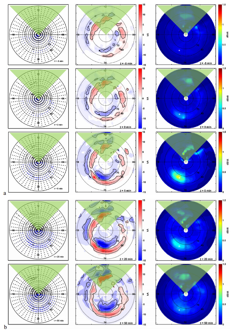
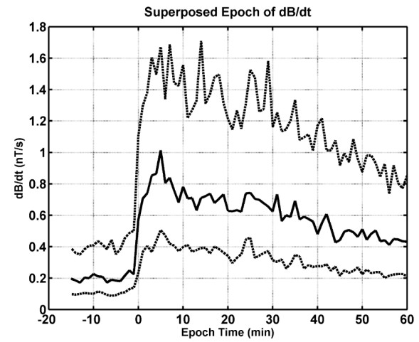
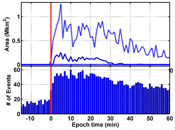
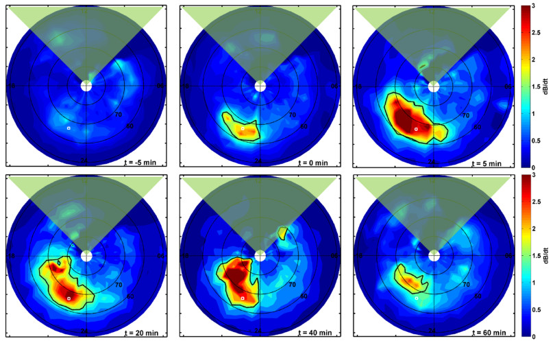
Ground induced currents (GICs) due to space weather are a threat to high voltage power transmission systems. However, knowledge of ground conductivity is the largest source of errors in the determination of GICs. A good proxy for GICs is dB/dt obtained from the Bx and By components of the magnetic field fluctuations. It is known that dB/dt values associated with magnetic storms can reach dangerous levels for power transmission systems. On the other hand, it is not uncommon for dB/dt values associated with substorms to exceed prior Pulkkinen and Molinski critical thresholds of 1.5 nT/s and 5 nT/s, respectively, and the temporal and spatial changes of the dB/dt associated with substorms, unlike storms, are not well understood. Using two dimensional maps of dB/dt over North America and Greenland derived from the spherical elementary currents, we investigate the temporal and spatial change of dB/dt for both a single substorm event and a two dimensional superposed epoch analysis of many substorms. Both the single event and the statistical analysis shows a sudden increase of dB/dt at substorm onset followed by an expansion poleward, westward, and eastward after the onset during the expansion phase. The area of dB/dt values exceeding the two critical thresholds from the initial onset dB/dt values showed little to no expansion equatorward. The temporal and spatial development of the dB/dt resembles the temporal and spatial change of the auroral emissions. Substorm values of dB/dt peak shortly after the auroral onset time and in at least one event exceeded 35 nT/s for a non-storm time substorm. In many of our 81 cases the area that exceeds the threshold of 1.5 nT/s is over several million square kilometers and after about 30 minutes the dB/dt values fall below the threshold level. These results address one of goals of the Space Weather Action Plan, which are to establish benchmarks for space weather events and improve modeling and prediction of their impacts on infrastructure. Plain language: The change in the ground magnetic field with respect to time (dB/dt) associated with magnetic storms (a large disturbance of the magnetic field of the earth) can reach dangerous levels for power transmission systems. On the other hand, substorms, which are a smaller more localized disturbance of the Earth's magnetic field, are more common. It is not uncommon for substorm dB/dt values to also exceed dangerous levels and the temporal and spatial changes of the dB/dt associated with substorms, unlike storms, are not well understood. Our analysis shows a sudden increase of dB/dt at substorm onset, which peaks shortly after the start of the substorm, followed shortly after by an expansion northward, westward, and eastward after the onset.
Citation: J.M. Weygand. The temporal and spatial development of dB/dt for substorms[J]. AIMS Geosciences, 2021, 7(1): 74-94. doi: 10.3934/geosci.2021004
Ground induced currents (GICs) due to space weather are a threat to high voltage power transmission systems. However, knowledge of ground conductivity is the largest source of errors in the determination of GICs. A good proxy for GICs is dB/dt obtained from the Bx and By components of the magnetic field fluctuations. It is known that dB/dt values associated with magnetic storms can reach dangerous levels for power transmission systems. On the other hand, it is not uncommon for dB/dt values associated with substorms to exceed prior Pulkkinen and Molinski critical thresholds of 1.5 nT/s and 5 nT/s, respectively, and the temporal and spatial changes of the dB/dt associated with substorms, unlike storms, are not well understood. Using two dimensional maps of dB/dt over North America and Greenland derived from the spherical elementary currents, we investigate the temporal and spatial change of dB/dt for both a single substorm event and a two dimensional superposed epoch analysis of many substorms. Both the single event and the statistical analysis shows a sudden increase of dB/dt at substorm onset followed by an expansion poleward, westward, and eastward after the onset during the expansion phase. The area of dB/dt values exceeding the two critical thresholds from the initial onset dB/dt values showed little to no expansion equatorward. The temporal and spatial development of the dB/dt resembles the temporal and spatial change of the auroral emissions. Substorm values of dB/dt peak shortly after the auroral onset time and in at least one event exceeded 35 nT/s for a non-storm time substorm. In many of our 81 cases the area that exceeds the threshold of 1.5 nT/s is over several million square kilometers and after about 30 minutes the dB/dt values fall below the threshold level. These results address one of goals of the Space Weather Action Plan, which are to establish benchmarks for space weather events and improve modeling and prediction of their impacts on infrastructure. Plain language: The change in the ground magnetic field with respect to time (dB/dt) associated with magnetic storms (a large disturbance of the magnetic field of the earth) can reach dangerous levels for power transmission systems. On the other hand, substorms, which are a smaller more localized disturbance of the Earth's magnetic field, are more common. It is not uncommon for substorm dB/dt values to also exceed dangerous levels and the temporal and spatial changes of the dB/dt associated with substorms, unlike storms, are not well understood. Our analysis shows a sudden increase of dB/dt at substorm onset, which peaks shortly after the start of the substorm, followed shortly after by an expansion northward, westward, and eastward after the onset.

| [1] |
Pulkkinen A (2017) Introduction to NASA Living With a Star (LWS) Institute GIC Working Group Special Collection. Space Weather 15: 738–740. doi: 10.1002/2016SW001537

|
| [2] | Piersanti M, Carter B (2020) Geomagnetically induced currents. The Dynamical Ionosphere. Elsevier, 121–134. |
| [3] |
Wei LH, Homeier N, Gannon JL (2013) Surface electric fields for North America during historical geomagnetic storms. Space Weather 11: 451–462. doi: 10.1002/swe.20073
|
| [4] | Kappenman JG (2010) Geomagnetic storms and their impacts on the U.S. power grid. Metatech-R-319, Oak Ridge, Tenn. |
| [5] |
Dimmock AP, Rosenqvist L, Welling DT, et al. (2020) On the regional variability of dB/dt and its significance to GIC. Space Weather 18: e2020SW002497. doi: 10.1029/2020SW002497
|
| [6] |
Rodger CJ, Mac Manus DH, Dalzell M, et al. (2017) Long-term geomagnetically induced current observations from New Zealand: Peak current estimates for extreme geomagnetic storms. Space Weather 15: 1447–1460. doi: 10.1002/2017SW001691
|
| [7] |
Stauning P (2013) Power grid disturbances and polar cap index during geomagnetic storms. J Space Weather Space Clim 3: A22. doi: 10.1051/swsc/2013044
|
| [8] |
Kappenman JG (2006) Great geomagnetic storms and extreme impulsive geomagnetic field disturbance events–An analysis of observational evidence including the great storm of May 1921. Adv Space Res 38: 188–199. doi: 10.1016/j.asr.2005.08.055
|
| [9] |
Pulkkinen A, Kuznetsova M, Ridley A, et al. (2011) Geospace Environment Modeling 2008–2009 Challenge: Ground magnetic field perturbations. Space Weather 9: S02004. doi: 10.1029/2010SW000600
|
| [10] |
Pulkkinen A, Rastätter L, Kuznetsova M, et al. (2013) Community-wide validation of geospace model ground magnetic field perturbation predictions to support model transition to operations. Space Weather 11: 369–385. doi: 10.1002/swe.20056
|
| [11] |
Molinski TS, Feero WE, Damsky BL (2000) Shielding grids from solar storms[power system protection]. IEEE Spectrum 37: 55–60. doi: 10.1109/6.880955
|
| [12] |
Molinski TS (2002) Why utilities respect geomagnetically induced currents. J Atmos Sol Terr Phys 64: 1765–1778. doi: 10.1016/S1364-6826(02)00126-8
|
| [13] | Piersanti M, Di Matteo S, Carter BA, et al. (2019) Geoelectric field evaluation during the September 2017 Geomagnetic Storm: MA. I. GIC. model. Space Weather 17: 1241–1256. |
| [14] |
Piersanti M, Michelis PD, Moro DD, et al. (2020) From the Sun to Earth: effects of the 25 August 2018 geomagnetic storm. Ann Geophys 38: 703–724. doi: 10.5194/angeo-38-703-2020
|
| [15] |
Minamoto Y, Fujita S, Hara M (2015) Frequency distributions of magnetic storms and SI+ SSC-derived records at Kakioka, Memambetsu, and Kanoya. Earth Planets Space 67: 1–6. doi: 10.1186/s40623-015-0362-4
|
| [16] | NOAA (2004) Halloween Space Weather Storms of 2003, NOAA Technical Memorandum OAR SEC-88. |
| [17] |
Ngwira CM, Sibeck D, Silveira MV, et al. (2018) A study of intense local dB/dt variations during two geomagnetic storms. Space Weather 16: 676–693. doi: 10.1029/2018SW001911
|
| [18] |
Pulkkinen A, Viljanen A, Pirjola R (2006) Estimation of geomagnetically induced current levels from different input data. Space Weather 4: S08005. doi: 10.1029/2006SW000229
|
| [19] | Bolduc L, Langlois P, Boteler D, et al. (1998) A study of geoelectromagnetic disturbances in Quebec. I. General results. IEEE Trans Power Delivery 13: 1251–1256. |
| [20] |
Blake SP, Gallagher PT, McCauley J, et al. (2016) Geomagnetically induced currents in the Irish power network during geomagnetic storms. Space Weather 14: 1136–1154. doi: 10.1002/2016SW001534
|
| [21] | Shelemy S (2012) Geomagnetically Induced Currents (GIC) And Manitoba Hydro. IEEE PES presentation. |
| [22] | Demetrescu C, Dobrica V, Greculeasa R, et al. (2018) The induced surface electric response in Europe to 2015 St. Patrick's Day geomagnetic storm. J Atmos Sol Terr Phys 180: 106–115. |
| [23] |
Borovsky JE, Nemzek RJ, Belian RD (1993) The occurrence rate of magnetospheric-substorm onsets: Random and periodic substorms. J Geophys Res Space Phys 98: 3807–3813. doi: 10.1029/92JA02556
|
| [24] |
McPherron RL, Chu X (2018) The midlatitude positive bay index and the statistics of substorm occurrence. J Geophys Res Space Phys 123: 2831–2850. doi: 10.1002/2017JA024766
|
| [25] | Akasofu SI (1964) The development of the auroral substorm. Planet Space Sci 2: 273–282. |
| [26] | Frey HU, Mende SB, Angelopoulos V, et al. (2004) Substorm onset observations by IMAGE-FUV. J Geophys Res Space Phys 109. |
| [27] |
Viljanen A, Tanskanen EI, Pulkkinen A (2006) Relation between substorm characteristics and rapid temporal variations of the ground magnetic field. Ann Geophys 24: 725–733. doi: 10.5194/angeo-24-725-2006
|
| [28] |
Amm O, Viljanen A (1999) Ionospheric disturbance magnetic field continuation from the ground to the ionosphere using spherical elementary current systems. Earth Planets Space 51: 431. doi: 10.1186/BF03352247
|
| [29] | Weygand JM (2009) Spherical Elementary Current (SEC) Amplitudes derived using the Spherical Elementary Currrent Systems (SECS) technique at 10 s Resolution in Geographic Coordinates, UCLA. Available from: https://doi.org/10.21978/P8PP8X. |
| [30] | Weygand JM, Amm O, Viljanen A, et al. (2011) Application and Validation of the Spherical Elementary Currents Systems Technique for Deriving Ionospheric Equivalent Currents with the North American and Greenland Ground Magnetometer Arrays. J Geophys Res Space Phys 116. |
| [31] |
Weygand JM, Kivelson MG, Frey HU, et al. (2015) An interpretation of spacecraft and ground based observations of multiple omega bands events. J Atmos Sol Terr Phys 13: 185–204. doi: 10.1016/j.jastp.2015.08.014
|
| [32] | Weygand JM (2009) Equivalent Ionospheric Currents (EICs) derived using the Spherical elementary Current Systems (SECS) technique at 10 s Resolution in Geographic Coordinates, UCLA. Available from: https://doi.org/10.21978/P8D62B. |
| [33] |
Donovan E, Mende S, Jackel B, et al. (2006) The THEMIS all-sky imaging array—System design and initial results from the prototype imager. J Atmos Sol Terr Phys 68: 1472–1487. doi: 10.1016/j.jastp.2005.03.027
|
| [34] | Mende SB, Harris SE, Frey HU, et al. (2008) The THEMIS array of ground-based observatories for the study of auroral substorms. In BurchV JL, Angelopoulos V, (eds), The THEMIS Mission, 357–387. |
| [35] |
Chu X, Hsu TS, McPherron RL, et al. (2014) Development and validation of inversion technique for substorm current wedge using ground magnetic field data. J Geophys Res Space Phys 119: 1909–1924. doi: 10.1002/2013JA019185
|
| [36] |
McPherron RL, Chu X (2017) The mid-latitude positive bay and the MPB index of substorm activity. Space Sci Rev 206: 91–122. doi: 10.1007/s11214-016-0316-6
|
| [37] | Engebretson MJ, Pilipenko VA, Ahmed LY, et al. (2019) Nighttime magnetic perturbation events observed in Arctic Canada: 1. Survey and statistical analysis. J Geophys Res Space Phys 124: 7442–7458. |
| [38] | Engebretson MJ, Steinmetz ES, Posch JL, et al. (2019) Nighttime magnetic perturbation events observed in Arctic Canada: 2. Multiple-instrument observations. J Geophys Res Space Phys 124: 7459–7476. |
| [39] |
Weygand JM, Wing S (2020) Temporal and spatial development of TEC enhancements during substorms. J Geophys Res Space Phys 125: e2019JA026985. doi: 10.1029/2019JA026985
|
 geosci-07-01-004-s001.pdf geosci-07-01-004-s001.pdf |
 |
Figures(8) / Tables(1)

J.M. Weygand. The temporal and spatial development of dB/dt for substorms[J]. AIMS Geosciences, 2021, 7(1): 74-94. doi: 10.3934/geosci.2021004


 DownLoad: