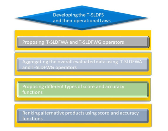
This paper aims to amalgamate the notion of a T-spherical fuzzy set (T-SFS) and a linear Diophantine fuzzy set (LDFS) to elaborate on the notion of the T-spherical linear Diophantine fuzzy set (T-SLDFS). The new concept is very effective and is more dominant as compared to T-SFS and LDFS. Then, we advance the basic operations of T-SLDFS and examine their properties. To effectively aggregate the T-spherical linear Diophantine fuzzy data, a T-spherical linear Diophantine fuzzy weighted averaging (T-SLDFWA) operator and a T-spherical linear Diophantine fuzzy weighted geometric (T-SLDFWG) operator are proposed. Then, the properties of these operators are also provided. Furthermore, the notions of the T-spherical linear Diophantine fuzzy-ordered weighted averaging (T-SLDFOWA) operator; T-spherical linear Diophantine fuzzy hybrid weighted averaging (T-SLDFHWA) operator; T-spherical linear Diophantine fuzzy-ordered weighted geometric (T-SLDFOWG) operator; and T-spherical linear Diophantine fuzzy hybrid weighted geometric (T-SLDFHWG) operator are proposed. To compare T-spherical linear Diophantine fuzzy numbers (T-SLDFNs), different types of score and accuracy functions are defined. On the basis of the T-SLDFWA and T-SLDFWG operators, a multiple attribute decision-making (MADM) method within the framework of T-SLDFNs is designed, and the ranking results are examined by different types of score functions. A numerical example is provided to depict the practicality and ascendancy of the proposed method. Finally, to demonstrate the excellence and accessibility of the proposed method, a comparison analysis with other methods is conducted.
Citation: Ashraf Al-Quran. T-spherical linear Diophantine fuzzy aggregation operators for multiple attribute decision-making[J]. AIMS Mathematics, 2023, 8(5): 12257-12286. doi: 10.3934/math.2023618
This paper aims to amalgamate the notion of a T-spherical fuzzy set (T-SFS) and a linear Diophantine fuzzy set (LDFS) to elaborate on the notion of the T-spherical linear Diophantine fuzzy set (T-SLDFS). The new concept is very effective and is more dominant as compared to T-SFS and LDFS. Then, we advance the basic operations of T-SLDFS and examine their properties. To effectively aggregate the T-spherical linear Diophantine fuzzy data, a T-spherical linear Diophantine fuzzy weighted averaging (T-SLDFWA) operator and a T-spherical linear Diophantine fuzzy weighted geometric (T-SLDFWG) operator are proposed. Then, the properties of these operators are also provided. Furthermore, the notions of the T-spherical linear Diophantine fuzzy-ordered weighted averaging (T-SLDFOWA) operator; T-spherical linear Diophantine fuzzy hybrid weighted averaging (T-SLDFHWA) operator; T-spherical linear Diophantine fuzzy-ordered weighted geometric (T-SLDFOWG) operator; and T-spherical linear Diophantine fuzzy hybrid weighted geometric (T-SLDFHWG) operator are proposed. To compare T-spherical linear Diophantine fuzzy numbers (T-SLDFNs), different types of score and accuracy functions are defined. On the basis of the T-SLDFWA and T-SLDFWG operators, a multiple attribute decision-making (MADM) method within the framework of T-SLDFNs is designed, and the ranking results are examined by different types of score functions. A numerical example is provided to depict the practicality and ascendancy of the proposed method. Finally, to demonstrate the excellence and accessibility of the proposed method, a comparison analysis with other methods is conducted.

| [1] | L. A. Zadeh, Fuzzy sets, Inform. Contr., 8 (1965), 338–353. |
| [2] | K. Atanassov, Intuitionistic fuzzy sets, Fuzzy Set. Syst., 20 (1986), 87–96. |
| [3] | R. R. Yager, Pythagorean fuzzy subsets, In: 2013 Joint IFSA World Congress NAFIPS Annual Meeting (IFSA/NAFIPS), 2013, 57–61. https://doi.org/10.1109/IFSA-NAFIPS.2013.6608375 |
| [4] |
R. R. Yager, Generalized orthopair fuzzy sets, IEEE T. Fuzzy Syst., 25 (2017), 1222–1230. https://doi.org/10.1109/TFUZZ.2016.2604005 doi: 10.1109/TFUZZ.2016.2604005

|
| [5] |
S. M. Chen, C. H. Chang, Fuzzy multi-attribute decision making based on transformation techniques of intuitionistic fuzzy values and intuitionistic fuzzy geometric averaging operators, Inform. Sci., 352 (2016), 133–149. https://doi.org/10.1016/j.ins.2016.02.049 doi: 10.1016/j.ins.2016.02.049
|
| [6] |
M. B. Khan, G. Santos-García, S. Treanțǎ, M. A. Noor, M. S. Soliman, Perturbed mixed variational-like inequalities and auxiliary principle pertaining to a fuzzy environment, Symmetry, 14 (2022), 2503. https://doi.org/10.3390/sym14122503 doi: 10.3390/sym14122503
|
| [7] |
A. K. Das, C. Granados, FP-intuitionistic multi fuzzy N-soft set and its induced FP-hesitant N soft set in group decision-making, Decis. Mak. Appl. Manag. Eng., 5 (2022), 67–89. https://doi.org/10.31181/dmame181221045d doi: 10.31181/dmame181221045d
|
| [8] |
R. R. Yager, Pythagorean membership grades in multicriteria decision making, IEEE T. Fuzzy Syst., 22 (2013), 958–965. https://doi.org/10.1109/TFUZZ.2013.2278989 doi: 10.1109/TFUZZ.2013.2278989
|
| [9] |
S. Abdullah, M. Qiyas, M. Naeem, Mamona, Y. Liu, Pythagorean cubic fuzzy Hamacher aggregation operators and their application in green supply selection problem, AIMS Math., 7 (2022), 4735–4766. https://doi.org/10.3934/math.2022263 doi: 10.3934/math.2022263
|
| [10] |
K. Kumar, S. M. Chen, Group decision making based on q-rung orthopair fuzzy weighted averaging aggregation operator of q-rung orthopair fuzzy numbers, Inform. Sciences, 598 (2022), 1–18. https://doi.org/10.1016/j.ins.2016.02.049 doi: 10.1016/j.ins.2016.02.049
|
| [11] |
M. Riaz, M. R. Hashmi, Linear Diophantine fuzzy set and its applications towards multi-attribute decision-making problems, J. Intell. Fuzzy Syst., 37 (2019), 5417–5439. https://doi.org/10.3233/JIFS-190550 doi: 10.3233/JIFS-190550
|
| [12] |
A. O. Almagrabi, S. Abdullah, M. Shams, Y. D. Al-Otaibi, S. Ashraf, A new approach to q-linear Diophantine fuzzy emergency decision support system for COVID-19, J. Amb. Intel. Hum. Comp., 13 (2022), 1687–1713. https://doi.org/10.1007/s12652-021-03130-y doi: 10.1007/s12652-021-03130-y
|
| [13] |
M. Riaz, H. M. A. Farid, M. Aslam, D. Pamucar, D. Bozanić, Novel approach for third-party reverse logistic provider selection process under linear Diophantine fuzzy prioritized aggregation operators, Symmetry, 13 (2021), 1152. https://doi.org/10.3390/sym13071152 doi: 10.3390/sym13071152
|
| [14] |
A. Iampan, G. S. Garcia, M. Riaz, H. Muhammad, A. Farid, R. Chinram, Linear Diophantine fuzzy Einstein aggregation operators for multi-criteria decision-making problems, J. Math., 2021 (2021). https://doi.org/10.1155/2021/5548033 doi: 10.1155/2021/5548033
|
| [15] |
T. Mahmood, I. Haleemzai, Z. Ali, D. Pamucar, D. Marinkovic, Power Muirhead mean operators for interval-valued linear Diophantine fuzzy sets and their application in decision-making strategies, Mathematics, 10 (2022), 70. https://doi.org/10.3390/math10010070 doi: 10.3390/math10010070
|
| [16] |
T. Mahmood, Z. Ali, K. Ullah, Q. Khan, A. Alsanad, M. A. A. Mosleh, Linear Diophantine uncertain linguistic power Einstein aggregation operators and their applications to multi attribute decision making, Complexity, 2021 (2021). https://doi.org/10.1155/2021/4168124 doi: 10.1155/2021/4168124
|
| [17] |
T. Mahmood, Z. Ali, M. Aslam, R. Chinram, Generalized Hamacher aggregation operators based on linear Diophantine uncertain linguistic setting and their applications in decision-making problems, IEEE Access, 9 (2021), 126748–126764. https://doi.org/10.1109/ACCESS.2021.3110273 doi: 10.1109/ACCESS.2021.3110273
|
| [18] |
M. Qiyas, M. Naeem, S. Abdullah, N. Khan, A. Ali, Similarity measures based on q-rung linear Diophantine fuzzy sets and their application in logistics and supply chain management, J. Math., 2022 (2022). https://doi.org/10.1155/2022/4912964 doi: 10.1155/2022/4912964
|
| [19] |
Z. Ali, T. Mahmood, G. Santos-García, Heronian mean operators based on novel complex linear Diophantine uncertain linguistic variables and their applications in multi-attribute decision making, Mathematics, 9 (2021), 2730. https://doi.org/10.3390/math9212730 doi: 10.3390/math9212730
|
| [20] |
H. Kamaci, Complex linear Diophantine fuzzy sets and their cosine similarity measures with applications, Complex Intell. Syst., 8 (2021), 1281–1305. https://doi.org/10.1007/s40747-021-00573-w doi: 10.1007/s40747-021-00573-w
|
| [21] |
H. Kamaci, Linear Diophantine fuzzy algebraic structures, J. Amb. Intell. Hum. Comput., 12 (2021), 10353–10373. https://doi.org/10.1007/s12652-020-02826-x doi: 10.1007/s12652-020-02826-x
|
| [22] |
S. Ayub, M. Shabir, M. Riaz, M. Aslam, R. Chinram, Linear Diophantine fuzzy relations and their algebraic properties with decision making, Symmetry, 13 (2021), 945. https://doi.org/10.3390/sym13060945 doi: 10.3390/sym13060945
|
| [23] |
M. Riaz, M. R. Hashmi, H. Kalsoom, D. Pamucar, Y. M. Chu, Linear Diophantine fuzzy soft rough sets for the selection of sustainable material handling equipment, Symmetry, 12 (2020), 1215. https://doi.org/10.3390/sym12081215 doi: 10.3390/sym12081215
|
| [24] |
K. Prakash, M. Parimala, H. Garg, M. Riaz, Lifetime prolongation of a wireless charging sensor network using a mobile robot via linear Diophantine fuzzy graph environment, Complex Intell. Syst., 8 (2022), 2419–2434. https://doi.org/10.1007/s40747-022-00653-5 doi: 10.1007/s40747-022-00653-5
|
| [25] |
M. Parimala, S. Jafari, M. Riaz, M. Aslam, Applying the Dijkstra algorithm to solve a linear Diophantine fuzzy environment, Symmetry, 13 (2021), 1616. https://doi.org/10.3390/sym13091616 doi: 10.3390/sym13091616
|
| [26] |
B. C. Cuong, Picture fuzzy sets, J. Comput. Sci. Cyb., 30 (2014), 409–420. http://dx.doi.org/10.15625/1813-9663/30/4/5032 doi: 10.15625/1813-9663/30/4/5032
|
| [27] |
M. W. Jang, J. H. Park, M. J. Son, Probabilistic picture hesitant fuzzy sets and their application to multi-criteria decision-making, AIMS Math., 8 (2023), 8522–8559. https://doi.org/10.3934/math.2023429 doi: 10.3934/math.2023429
|
| [28] |
A. Ashraf, K. Ullah, A. Hussain, M. Bari, Interval-valued picture fuzzy Maclaurin symmetric mean operator with application in multiple attribute decision-making, Rep. Mech. Eng., 3 (2022), 210–226. https://doi.org/10.31181/rme20020042022a doi: 10.31181/rme20020042022a
|
| [29] |
B. F. Yildirim, S. K. Yıldırım, Evaluating the satisfaction level of citizens in municipality services by using picture fuzzy VIKOR method: 2014-2019 period analysis, Decis. Mak. Appl. Manag. Eng., 5 (2022), 50–66. https://doi.org/10.31181/dmame181221001y doi: 10.31181/dmame181221001y
|
| [30] |
S. Ashraf, S. Abdullah, T. Mahmood, F. Ghani, T. Mahmood, Spherical fuzzy sets and their applications in multi-attribute decision making problems, J. Intell. Fuzzy Syst., 36 (2019), 2829–2844. https://doi.org/10.3233/JIFS-172009 doi: 10.3233/JIFS-172009
|
| [31] |
T. Mahmood, K. Ullah, Q. Khan, N. Jan, An approach toward decision-making and medical diagnosis problems using the concept of spherical fuzzy sets, Neural Comput. Appl., 31 (2019), 7041–7053. https://doi.org/10.1007/s00521-018-3521-2 doi: 10.1007/s00521-018-3521-2
|
| [32] |
Z. Ali, T. Mahmood, M. S. Yang, TOPSIS method based on complex spherical fuzzy sets with Bonferroni mean operators, Mathematics, 8 (2020), 1739. https://doi.org/10.3390/math8101739 doi: 10.3390/math8101739
|
| [33] |
M. Qiyas, M. Naeem, S. Abdullah, N. Khan, Decision support system based on complex T-Spherical fuzzy power aggregation operators, AIMS Math., 7 (2022), 16171–16207. https://doi.org/10.3934/math.2022884 doi: 10.3934/math.2022884
|
| [34] |
S. G. Quek, G. Selvachandran, M. Munir, T. Mahmood, K. Ullah, L. H. Son, et al., Multi-attribute multi-perception decision-making based on generalized T-spherical fuzzy weighted aggregation operators on neutrosophic sets, Mathematics, 7 (2019), 780. https://doi.org/10.3390/math7090780 doi: 10.3390/math7090780
|
| [35] |
A. Al-Quran, A new multi attribute decision making method based on the T-spherical hesitant fuzzy sets, IEEE Access, 9 (2021), 156200–156210. https://doi.org/10.1109/ACCESS.2021.3128953 doi: 10.1109/ACCESS.2021.3128953
|
| [36] |
H. Garg, K. Ullah, T. Mahmood, N. Hassan, N. Jan, T-spherical fuzzy power aggregation operators and their applications in multi-attribute decision making, J. Amb. Intel. Hum. Comput., 12 (2021), 9067–9080. https://doi.org/10.1007/s12652-020-02600-z doi: 10.1007/s12652-020-02600-z
|
| [37] |
M. Naeem, A. Khan, S. Ashraf, S. Abdullah, M. Ayaz, N. Ghanmi, A novel decision making technique based on spherical hesitant fuzzy Yager aggregation information: Application to treat Parkinson's disease, AIMS Math., 7 (2022), 1678–1706. https://doi.org/10.3934/math.2022097 doi: 10.3934/math.2022097
|
| [38] |
K. Ullah, H. Garg, T. Mahmood, N. Jan, Z. Ali, Correlation coefficients for T-spherical fuzzy sets and their applications in clustering and multi-attribute decision making, Soft Comput., 24 (2020), 1647–1659. https://doi.org/10.1007/s00500-019-03993-6 doi: 10.1007/s00500-019-03993-6
|
| [39] |
Y. Chen, M. Munir, T. Mahmood, A. Hussain, S. Zeng, Some generalized T-spherical and group-generalized fuzzy geometric aggregation operators with application in MADM problems, J. Math., 2021 (2021). https://doi.org/10.1155/2021/5578797 doi: 10.1155/2021/5578797
|
| [40] |
F. Karaaslan, M. A. D. Dawood, Complex T-spherical fuzzy Dombi aggregation operators and their applications in multiple-criteria decision-making, Complex Intell. Syst., 7 (2021), 2711–2734. https://doi.org/10.1007/s40747-021-00446-2 doi: 10.1007/s40747-021-00446-2
|
| [41] |
P. Liu, B. Zhu, P. Wang, A multi-attribute decision-making approach based on spherical fuzzy sets for Yunnan Baiyao's R$ & $D project selection problem, Int. J. Fuzzy Syst., 21 (2019), 2168–2191. https://doi.org/10.1007/s40815-019-00687-x doi: 10.1007/s40815-019-00687-x
|
| [42] |
P. Liu, B. Zhu, P. Wang, M. Shen, An approach based on linguistic spherical fuzzy sets for public evaluation of shared bicycles in China, Eng. Appl. Artif. Intell., 87 (2020), 103295. https://doi.org/10.1016/j.engappai.2019.103295 doi: 10.1016/j.engappai.2019.103295
|
| [43] |
M. Q. Wu, T. Y. Chen, J. P. Fan, Divergence measure of T-spherical fuzzy sets and its applications in pattern recognition, IEEE Access, 8 (2020), 10208–10221. https://doi.org/10.1109/ACCESS.2019.2963260 doi: 10.1109/ACCESS.2019.2963260
|
| [44] |
P. Devi, B. Kizielewicz, A. Guleria, A. Shekhovtsov, J. Wątróbski, T. Królikowski, et al., Decision support in selecting a reliable strategy for sustainable Urban transport based on Laplacian energy of T-spherical fuzzy graphs, Energies, 15 (2022), 4970. https://doi.org/10.3390/en15144970 doi: 10.3390/en15144970
|
| [45] |
M. Riaz, M. R. Hashmi, D. Pamucar, Y. Chu, Spherical linear Diophantine fuzzy sets with modeling uncertainties in MCDM, Comput. Model. Eng. Sci., 126 (2021), 1125–1164. https://doi.org/10.32604/cmes.2021.013699 doi: 10.32604/cmes.2021.013699
|
Figures(4) / Tables(7)

Ashraf Al-Quran. T-spherical linear Diophantine fuzzy aggregation operators for multiple attribute decision-making[J]. AIMS Mathematics, 2023, 8(5): 12257-12286. doi: 10.3934/math.2023618


 DownLoad: