Loading [MathJax]/jax/output/SVG/jax.js
Research article Special Issues

Unsaturated behavior of excavations in residual soil at the Auburn University National Geotechnical Experimentation Site

  • Two excavations were instrumented at the Auburn National Geotechnical Experimentation Site (NGES) in Opelika, AL. The excavations were constructed approximately 6 m deep × 30 m long with a vertical face. The primary goal of this experiment was to determine the boundary conditions that resulted in failure of the excavation. In doing so, conclusions were drawn regarding the accuracy of common laboratory test methods for estimating the strength properties of residual soil.
    The instrumentation plan was designed to monitor real-time pore water pressures (positive and negative) surrounding the excavation throughout the course of each 1-year test period. Time-lapse cameras were used to identify when failures occurred, and the approximate geometry of the failure planes. Undisturbed soil samples were taken during the subsurface exploration and used in conjunction with previous soil test results to accurately define the material properties and layering based on common laboratory test methods. In addition to common laboratory tests, unsaturated triaxial tests were also conducted, and soil-water characteristic curves were measured to further define the unsaturated properties of the soil.
    In both excavations, failure was observed along a similar plane, which began at the bottom of the excavation, and propagated to the surface (approximately 2 m behind the face of the excavation) along existing tension cracks that developed during the construction of the excavation. Based on these results, recommendations are provided as related to the most appropriate test methods for determining the strength properties of residual soil for use in geotechnical design.

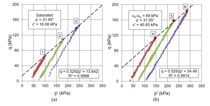
    Citation: Richard E. Burrage, J. Brian Anderson. Unsaturated behavior of excavations in residual soil at the Auburn University National Geotechnical Experimentation Site[J]. AIMS Geosciences, 2019, 5(4): 921-939. doi: 10.3934/geosci.2019.4.921

    Related Papers:

    [1] Travis G. Draper, Fernando Guevara Vasquez, Justin Cheuk-Lum Tse, Toren E. Wallengren, Kenneth Zheng . Matrix valued inverse problems on graphs with application to mass-spring-damper systems. Networks and Heterogeneous Media, 2020, 15(1): 1-28. doi: 10.3934/nhm.2020001
    [2] Sergei Avdonin, Julian Edward . An inverse problem for quantum trees with observations at interior vertices. Networks and Heterogeneous Media, 2021, 16(2): 317-339. doi: 10.3934/nhm.2021008
    [3] Robert Carlson . Dirichlet to Neumann maps for infinite quantum graphs. Networks and Heterogeneous Media, 2012, 7(3): 483-501. doi: 10.3934/nhm.2012.7.483
    [4] Franco Cardin, Alberto Lovison . Finite mechanical proxies for a class of reducible continuum systems. Networks and Heterogeneous Media, 2014, 9(3): 417-432. doi: 10.3934/nhm.2014.9.417
    [5] Luis Caffarelli, Antoine Mellet . Random homogenization of fractional obstacle problems. Networks and Heterogeneous Media, 2008, 3(3): 523-554. doi: 10.3934/nhm.2008.3.523
    [6] Luca Placidi, Julia de Castro Motta, Rana Nazifi Charandabi, Fernando Fraternali . A continuum model for the tensegrity Maxwell chain. Networks and Heterogeneous Media, 2024, 19(2): 597-610. doi: 10.3934/nhm.2024026
    [7] Manuel Friedrich, Bernd Schmidt . On a discrete-to-continuum convergence result for a two dimensional brittle material in the small displacement regime. Networks and Heterogeneous Media, 2015, 10(2): 321-342. doi: 10.3934/nhm.2015.10.321
    [8] Delio Mugnolo . Gaussian estimates for a heat equation on a network. Networks and Heterogeneous Media, 2007, 2(1): 55-79. doi: 10.3934/nhm.2007.2.55
    [9] Bernd Schmidt . On the derivation of linear elasticity from atomistic models. Networks and Heterogeneous Media, 2009, 4(4): 789-812. doi: 10.3934/nhm.2009.4.789
    [10] Fermín S. V. Bazán, Luciano Bedin, Mansur I. Ismailov, Leonardo S. Borges . Inverse time-dependent source problem for the heat equation with a nonlocal Wentzell-Neumann boundary condition. Networks and Heterogeneous Media, 2023, 18(4): 1747-1771. doi: 10.3934/nhm.2023076
  • Two excavations were instrumented at the Auburn National Geotechnical Experimentation Site (NGES) in Opelika, AL. The excavations were constructed approximately 6 m deep × 30 m long with a vertical face. The primary goal of this experiment was to determine the boundary conditions that resulted in failure of the excavation. In doing so, conclusions were drawn regarding the accuracy of common laboratory test methods for estimating the strength properties of residual soil.
    The instrumentation plan was designed to monitor real-time pore water pressures (positive and negative) surrounding the excavation throughout the course of each 1-year test period. Time-lapse cameras were used to identify when failures occurred, and the approximate geometry of the failure planes. Undisturbed soil samples were taken during the subsurface exploration and used in conjunction with previous soil test results to accurately define the material properties and layering based on common laboratory test methods. In addition to common laboratory tests, unsaturated triaxial tests were also conducted, and soil-water characteristic curves were measured to further define the unsaturated properties of the soil.
    In both excavations, failure was observed along a similar plane, which began at the bottom of the excavation, and propagated to the surface (approximately 2 m behind the face of the excavation) along existing tension cracks that developed during the construction of the excavation. Based on these results, recommendations are provided as related to the most appropriate test methods for determining the strength properties of residual soil for use in geotechnical design.


    Fractional derivatives and integrals are generalization of derivatives and integrals to arbitrary non-integer orders. The theory of fractional calculus has been studied and applied to be valuable tools in the investigation and explanation of many phenomena in various fields such as chemistry, physics [1,2], engineering [3], economics [4], control theory [5], epidemiology [6,8,7], etc (see [10,11,9]). Differential equations involving time-fractional derivatives are more realistic to explain some phenomena than those of integer order in time because it can describe the rate of change that depends on the past state. Consequently, fractional derivatives have been investigated on qualitative and numerical aspects [12,13] for describing physical phenomena.

    There are various definitions of fractional derivatives and integrals, which include Riemann-Liouville, Caputo, Hilfer, Riesz, Erdelyi-Kober, Hadamard, etc [11,1,10,9]. Among these definitions, Caputo derivative and Riemann-Liouville are widely used by many researchers. In addition, they are derived from the corresponding fractional integral operators. The variation of fractional calculus in many different forms of fractional derivative and integral operators arises from various special functions. In one direction, the integral operators have been extended to include the weight function φ as a definition of generalized Caputo fractional derivative by Almeida [14]. This definition has the advantage in terms of accuracy in mathematical modeling if a function φ is appropriately selected. Later, Jarad and Abdeljawad [15] constructed the Laplace transform and its inverse operator which depends on another function φ for solving some fractional differential systems in the notion of φ-Caputo fractional derivative.

    Over the past years, there has been an essential development in fractional evolution equations since many problems occurring in science, engineering and economy can be formulated by fractional evolution equations. Evolution equations are generally used to interpret the changing and evolving over time of the system. For instance, reaction-diffusion equations in chemical physics and biology [16,17], Schrödinger equations in quantum mechanics [18,19], Navier-Stokes equation in fluid mechanics [20], and Black-Scholes equation in finance [21] are common examples of fractional evolution equations. The development in the theory of fractional evolution equations is an essential branch of fractional calculus ranging from the study of existence, uniqueness, stability [22,23], numerical techniques [24] and mathematical modeling [26,25]. In particular, the existence and uniqueness theorems for fractional evolution equations have been extensively studied by means of semigroup theory and fixed point theorems [24,27,28,29,30,31,32,33,34,35,36].

    Various types of fixed point theorems are extensively used as fundamental tools for proving the existence and uniqueness of solutions for fractional evolution equations. However, some fixed point theorems are non-constructive results. As we all know, the monotone iterative method [37] is a flexible and efficient technique that provides both existence and constructive results for nonlinear differential equations [38,39,40,42,41,43] in terms of the lower and upper solutions. Furthermore, it can contribute to several comparison results which are applicable tools for the study. In this work, we emphasize on using the monotone iterative method involving the construction of upper and lower solutions.

    In 2020, Gou and Li [44] investigated the existence and uniqueness of mild solutions for impulsive fractional evolution equations of Volterra and Fredholm types in an ordered Banach space E subject to the periodic boundary condition by means of monotone iterative method for the problem

    {CDα0u(t)+Au(t)=f(t,u(t),Gu(t),Hu(t)),tJ,ttkΔu|t=tk=Ik(u(tk)),k=1,2,,m,u(0)=u(ω)

    where CDα0 is the classical Caputo fractional derivative of order 0<α<1 with the lower limit zero, A:D(A)EE is a closed linear operator and A generates a C0semigroup {T(t)}t0 in E; fC(J×E×E×E,E) is a function, IkC(E,E) is an impulsive function, k=1,2,,m; J=[0,ω], J=J{t1,t2,,tm}, J0=[0,t1], Jk=(tk,tk+1], the {tk} satisfy 0=t0<t1<t2<<tm<tm+1=ω, mN; Δu(tk)=u(t+k)u(tk), u(t+k) and u(tk) represent the right and left limits of u(t) at t=tk, respectively. The operators G and H are Volterra integral operator and Fredholm integral operator, respectively, which are defined by

    Gu(t)=t0g(t,s)u(s)ds (1.1)

    where the integral kernel gC(Ω,R+) and Ω={(t,s)R2|0stT}, and

    Hu(t)=T0h(t,s)u(s)ds (1.2)

    with the integral kernel hC(¯Ω,R+) and ¯Ω={(t,s)R2|0t,sT}.

    Recently, Derbazi et al. [45] studied the existence and uniqueness of extremal solutions for fractional differential equations involving the φCaputo derivative subject to an initial condition:

    {CDα;φau(t)=f(t,u(t)),t[a,b]u(a)=a

    where CDα;φa is the φCaputo fractional derivative of order 0<α<1, f:[a,b]×RR is a given continuous function and aR.

    Inspired by [44,45], some monotone conditions and noncompactness measure conditions of nonlinearity f, we use the monotone iterative technique to establish the existence of solutions of fractional evolution equations in an order Banach space E given by

    {CDα;φt0u(t)=Au(t)+f(t,u(t),Gu(t),Hu(t)),t>t0u(t0)=u0 (1.3)

    where 0<α<1, 0t0tT< and u0E. Here A:D(A)EE is the infinitesimal generator of an analytic semigroup of uniformly bounded linear operators {T(t)}t0 on E. The nonlinearity f:[t0,T]×E×E×EE is a function involving the Volterra integral operator G and the Fredholm integral operator H defined by

    Gu(t)=tt0g(t,s)u(s)ds (1.4)

    where the integral kernel gC(Ω,R+) and Ω={(t,s)R2|t0stT}, and

    Hu(t)=Tt0h(t,s)u(s)ds (1.5)

    with the integral kernel hC(¯Ω,R+) and ¯Ω={(t,s)R2|t0t,sT}.

    The motivation for this work is taken by Derbazi et al. [45] and we apply the same techniques used in [45]. However, the generalization of this problem to our work involves evolution operator A. Hence, in order to establish the existence of solutions, it is required to derive the form of fundamental solution in terms of a semigroup induced by resolvent with respect to the weight function φ. Moreover, we notice that our problem (1.3) can be reduced to the work of Derbazi et al. [45] when the evolution operator A, and the operators G and H are taken to be zero operators on Banach space E=R.

    In this paper, we aim to derive a mild solution for the problem (1.3) in terms of semigroup depending on a function φ from Caputo fractional derivative. In addition, we construct lower and upper solutions to prove the existence and uniqueness results of mild solution for the problem (1.3) under the condition that {T(t)}t0 do not require compactness by using the monotone iterative technique. Moreover, the results obtained in this work are in the abstract form based on a more general definition of φCaputo fractional derivative so that it can be extended and generalized some results in the literature such as the impulsive evolution equations [44,42], the evolution equations with delay and nonlocal conditions.

    This manuscript is organized as follows. In Section 2, we recall basic concepts for fractional calculus and some known results used in the later. In section 3, we construct a mild solution of the Cauchy problem (1.3) in the form of operator semigroup involving a function φ which is obtained from the generalized Caputo derivative and then give the definitions of lower and upper solutions. Next, we investigate the existence and uniqueness results of mild solutions for the Cauchy problem (1.3) under the assumption that {T(t)}t0 does not require compactness by using the monotone iterative method in Section 4. Moreover, we provide an example to illustrate the results obtained in Section 5 and conclusion in Section 6.

    In this section, we recall some notations and definitions of fractional calculus and give auxiliary results which will be used in the sequel.

    We begin by introducing some properties of cones on real Banach spaces E.

    In cone P, a partially ordered is defined which means if xy if and only if yxP. If xy and xy, then we denote x<y or y>x.

    Definition 2.1. [46] The cone P is called

    (N) normal if there exists a constant N>0 such that x1Nx2 if θx1x2, for all x1,x2E. The least positive number satisfying above is called the normal constant of P.

    (R) regular if every increasing sequence which is bounded from above is convergent. That is, if {xn}n1 is a sequence such that

    x1x2y

    for some yE, then there is xE such that limnxnx=0.

    Lemma 2.2. [46,47]

    (i). Every regular cone is normal.

    (ii). The cone P is regular if and only if every decreasing sequence which is bounded from below is convergent.

    Theorem 2.3. [48] Let E be a weakly complete Banach space and P a cone in E. Then, P is normal if and only if P is regular.

    Definition 2.4. An operator family S(t)(t0) is said to be a positive operator in E if for any uP and t0 such that S(t)uθ.

    Here, we assume that E is an ordered Banach space with the norm and the partial order , whose positive cone P={xE:xθ} (θ is the zero element of E) is normal with normal constant N>0.

    Let C([t0,T],E) be the Banach space of all continuous maps from [t0,T] to E with the norm uC=supt[t0,T]u(t). For x1,x2C([t0,T],E), x1x2 if and only if x1(t)x2(t) for all t[t0,T]. For v,wC([t0,T],E), denote the ordered interval [v,w]={uC([t0,T],E):vuw} and [v(t),w(t)]={uE:v(t)uw(t)} for all t[t0,T].

    Next, we briefly highlight the definition and some basic properties of the φCaputo fractional derivative which are used throughout this paper.

    Definition 2.5. (φ-Riemann-Liouville fractional integral, [14]) Let α>0, uL1([a,b]) and φC1([a,b]) be a function such that φ(t)>0 for all t[a,b]. The φ-Riemann-Liouville fractional integral of order α of a function u with respect to another function φ is defined by

    (Iα;φau)(t)=1Γ(α)ta(φ(t)φ(s))α1u(s)φ(s)ds. (2.1)

    The above definition can be reduced to the classical Riemann-Liouville fractional integral when φ(t)=t.

    Definition 2.6. (φ-Riemann-Liouville fractional derivative, [14] ) Let α>0, nN and u,φCn([a,b]) be two functions such that φ(t)>0, for all t[a,b]. The φ-Riemann-Liouville fractional derivative of a function u of order α is defined by

    (Dα;φau)(t)=(1φ(t)ddt)n(Inα;φau)(t)=1Γ(nα)(1φ(t)ddt)nta(φ(t)φ(s)nα1u(s)φ(s)ds

    where n=[α]+1.

    Definition 2.7. (φ-Caputo fractional derivative, [14,15]) Let α>0, nN and u,φCn([a,b]) be two functions such that φ(t)>0 for all t[a,b]. The φ-Caputo fractional derivative of a function u of order α is defined by

    (CDα;φau)(t)=(Inα;φau[n])(t)=1Γ(nα)ta(φ(t)φ(s))nα1u[n](s)φ(s)ds

    where n=[α]+1 and u[n](t):=(1φ(t)ddt)nu(t) on [a,b].

    Lemma 2.8. [14] Let α>0. If uCn([a,b]) then

    Iα;φa(CDα;φau(t))=u(t)n1k=0u[k](a+)k!(φ(t)φ(a))k.

    In particular, given α(0,1), we have

    Iα;φa(CDα;φau(t))=u(t)u(a).

    Definition 2.9. [15] Let u and φ be real valued functions on [a,) such that φ(t) is continuous and φ(t)>0 on [a,). The generalized Laplace transform of u is defined by

    Lφ{u(t)}(s)=aes(φ(t)φ(a))u(t)φ(t)dt

    for all s.

    Definition 2.10. [15] Let u and v be piecewise continuous functions on an interval [a,b] and of exponential order. The generalized convolution of u and v is defined as

    (uφv)(t)=tau(τ)v(φ1(φ(t)+φ(a)φ(τ)))φ(τ)dτ.

    Theorem 2.11. (Gronwall’s inequality, [49,50]) Let φC1([a,b]) be a function such that φ(t)>0 for all t[a,b]. Suppose that

    (i) u and v are nonnegative and integrable functions;

    (ii) w is nonnegative continuous and nondecreasing function on [a,b]

    with

    u(t)v(t)+w(t)ta(φ(t)φ(s))α1u(s)φ(s)ds.

    Then

    u(t)v(t)+tak=1[w(t)Γ(α)]kΓ(nα)(φ(t)φ(s))kα1v(s)φ(s)ds

    for all t[a,b].

    Definition 2.12. [51,52] Let 0<α<1 and zC. The function ϕα defined by

    ϕα(z)=k=0(z)kk!Γ(αk+1α)=1πk=0(z)kΓ(α(k+1))sin(π(k+1)α)k!

    is called Wright type function.

    Proposition 2.13. [51,52] The Wright type function ϕα is an entire function and has the following properties:

    (i) ϕα(θ)0 for θ0 and 0ϕα(θ)dθ=1;

    (ii) 0ϕα(θ)θrdθ=Γ(1+r)Γ(1+αr) \quad for r>1;

    (iii) 0ϕα(θ)ezθdθ=Eα(z),zC;

    (iv) α0θϕα(θ)ezθdθ=Eα,α(z),zC

    where Eα(z)=k=0zkΓ(kα+1) is the Mittag-Leffler function with zC and α>0.

    Now, we recall the definition and some properties of Kuratowski measure of noncompactness.

    Definition 2.14. [53] Let B be a bounded set of Banach space E. The Kuratowski measure of noncompactness μ() is defined by

    μ(B):=inf{ε>0:Bni=1Bj,diam(Bi)<ε}

    where diam(Bi)=sup{|yx|:x,yBi} for i=1,2,nN.

    Lemma 2.15. [54] Let C and D be bounded subsets of a Banach space E. The noncompactness measure which satisfies the following properties:

    (i) D is precompact if and only if μ(D)=0;

    (ii) μ(CD)=max{μ(C),μ(D)} ;

    (iii) μ(C+D)μ(C)+μ(D);

    (iv) μ(λC)=|λ|μ(C) where λR;

    (v) Let X be another Banach space. If S:D(S)EX satisfies Lipschitz continuity with constant L, then

    μ(S(B))Lμ(B)

    for any bounded subset BD(S).

    Lemma 2.16. [54] If BC([t0,T],E) is bounded and equicontinuity, then μ(B(t)) is continuous on [t0,T], and

    μ(B)=supt[t0,T]μ(B(t))

    where B(t)={u(t):uB} for all t[t0,T].

    Lemma 2.17. [55] If BC([t0,T],E) is bounded and equicontinuous, then μ(B(t)) is continuous on [t0,T], and

    μ({Tt0u(t)dt|uB})Tt0μ(B(t))dt.

    Lemma 2.18. [56] If B={un}n=1C([t0,T],E) be a bounded and countable set, then μ(B(t)) is Lebesgue integral on [t0,T], and

    μ({Tt0un(t)dtnN})2Tt0μ(B(t))dt.

    Throughout this work, A is assumed to be the infinitesimal generator of a strongly continuous semigroup (i.e., C0-semigroup) of uniformly bounded linear operators {T(t)}t0 on E with

    M=supt[0,)T(t)for some M1.

    In this section, we derive the mild solution of the Cauchy problem (1.3) based on the semigroup theory and generalized Laplace transform.

    Lemma 3.1. Assume vC([t0,T],E) and 0<α<1. The mild solution of the linear Cauchy problem

    {CDα;φt0u(t)=Au(t)+v(t),t>t0u(t0)=u0E (3.1)

    is given by

    u(t)=Sα;φ(t,t0)u0+tt0(φ(t)φ(s))α1Tα;φ(t,s)v(s)φ(s)ds,t[t0,T] (3.2)

    where the operators Sα;φ(t,s) and Tα;φ(t,s) are defined by

    Sα;φ(t,s)u=0ϕα(θ)T((φ(t)φ(s))αθ)udθ (3.3)

    and

    Tα;φ(t,s)u=α0θϕα(θ)T((φ(t)φ(s))αθ)udθ (3.4)

    for 0stT and uE.

    Proof. The proof follows similar ideas as in [57]. Firstly, we apply the Definition 2.7 and Lemma 2.8 into the Cauchy problem (3.1). It can be rewritten the Cauchy problem (3.1) in form of the integral representation as

    u(t)=u0+1Γ(α)tt0(φ(t)φ(τ))α1(Au(τ)+v(τ))φ(τ)dτ. (3.5)

    Taking the generalized Laplace transforms to both sides of (3.5), we get that for λ>0,

    U(λ)=λα1(λαIA)1u0+(λαIA)1V(λ)=λα10eλαsT(s)u0ds+0eλαsT(s)V(λ)ds=α0(λη)α1e(λη)αT(ηα)u0dη+α0ηα1e(λη)αT(ηα)V(λ)dη=:J1+J2

    where

    U(λ)=t0eλ(φ(τ)φ(t0))u(τ)φ(τ)dτ

    and

    V(λ)=t0eλ(φ(τ)φ(t0))v(τ)φ(τ)dτ.

    Substituting η=φ(t)φ(t0) into J1 and J2 gives

    J1=αt0λα1(φ(t)φ(t0))α1e(λ(φ(t)φ(t0)))αT((φ(t)φ(t0))α)u0φ(t)dt=t01λddt(e(λ(φ(t)φ(t0)))α)T((φ(t)φ(t0))α)u0dt

    and

    J2=t0α(φ(t)φ(t0))α1e(λ(φ(t)φ(t0)))α×T((φ(t)φ(t0))α)V(λ)φ(t)dt=t0t0α(φ(t)φ(t0))α1e(λ(φ(t)φ(t0)))α×T((φ(t)φ(t0))α)e(λ(φ(s)φ(t0)))v(s)φ(s)φ(t)dsdt.

    The following one-sided stable probability density in [2] is considered by

    ρα(θ)=1πk=1(1)k1θαk1Γ(αk+1)k!sin(kπα),θ(0,)

    whose integration is given by

    0eλθρα(θ)dθ=eλαfor0<α<1. (3.6)

    Applying (3.6) to J1 and J2, it follows that

    J1=t00θρα(θ)eλ(φ(t)φ(t0))θT((φ(t)φ(t0))α)u0φ(t)dθdt=t0eλ(φ(t)φ(t0))(0ρα(θ)T((φ(t)φ(t0))αθα)u0dθ)φ(t)dt

    and

    J2=t0t00α(φ(t)φ(t0))α1ρα(θ)eλ(φ(t)φ(t0))θ×T((φ(t)φ(t0))α)eλ(φ(s)φ(t0))v(s)φ(s)φ(t)dθdsdt=t0t00αeλ(φ(t)+φ(s)2φ(t0))(φ(t)φ(t0))α1θαρα(θ)×T((φ(t)φ(t0))αθα)v(s)φ(s)φ(t)dθdsdt=t0t0αeλ(φ(τ)φ(t0))ρα(θ)(φ(t)φ(t0))α1θα×T((φ(t)φ(t0))αθα)v(φ1(φ(τ)φ(t)+φ(t0)))φ(τ)φ(t)dθdτdt=t0τt00αeλ(φ(τ)φ(t0))ρα(θ)(φ(t)φ(t0))α1θα×T((φ(t)φ(t0))αθα)v(φ1(φ(τ)φ(t)+φ(t0)))φ(τ)φ(t)dθdtdτ=t0eλ(φ(τ)φ(t0))×(τt00αρα(θ)(φ(τ)φ(s))α1θαT((φ(τ)φ(s))αθα)v(s)φ(s)dθds)φ(τ)dτ.

    It follows that

    U(λ)=t0eλ(φ(t)φ(t0))(0ρα(θ)T((φ(t)φ(t0))αθα)u0dθ)φ(t)dt+t0eλ(φ(τ)φ(t0))×(τt00αρα(θ)(φ(τ)φ(s))α1θαT((φ(τ)φ(s))αθα)v(s)φ(s)dθds)φ(τ)dτ.

    Hence, we apply the inverse Laplace transform to get

    u(t)=0ρα(θ)T((φ(t)φ(t0))αθα)u0dθ+tt00αρα(θ)(φ(t)φ(s))α1θαT((φ(t)φ(s))αθα)v(s)φ(s)dθds=0ϕα(θ)T((φ(t)φ(t0))αθ)u0dθ+tt0(φ(t)φ(s))α1(0αθϕα(θ)T((φ(t)φ(t0))αθ)dθ)v(s)φ(s)ds:=Sα;φ(t,t0)u0+tt0(φ(t)φ(s))α1Tα;φ(t,s)v(s)φ(s)ds

    where ϕα(θ)=1αθ11αρα(θ1α) is the probability density function defined on (0,).

    Lemma 3.2. [57] The operators Sα;φ and Tα;φ have the following properties:

    (i) For any fixed 0st, Sα;φ(t,s) and Tα;φ(t,s) are bounded linear operators with

    Sα;φ(t,s)(u)MuandTα;φ(t,s)(u)αMΓ(1+α)u=MΓ(α)u

    for all uE.

    (ii) The operators Sα;φ(t,s) and Tα;φ(t,s) are strongly continuous for all 0st, that is, for every uE and 0st1<t2T we have

    Sα;φ(t2,s)uSα;φ(t1,s)u0andTα;φ(t2,s)uTα;φ(t1,s)u0

    as t1t2.

    Definition 3.3. A function uC([t0,T],E) is called a mild solution of (1.3) if it satisfies

    u(t)=Sα;φ(t,t0)u0+tt0(φ(t)φ(s))α1Tα;φ(t,s)f(s,u(s),Gu(s),Hu(s))φ(s)ds

    where the operators Sα;φ and Tα;φ are defined by (3.3) and (3.4), respectively.

    From Definition 2.4, if T(t)(t0) is a positive semigroup generated by A, f and u0 are nonnegaive, then the mild solution uC([t0,T],E) of Cauchy problem (1.3) satisfies uθ.

    Definition 3.4. A function u_C([t0,T],E) is called a lower solution of problem (1.3) and satisfies

    {CDα;φt0u_(t)Au_(t)+f(t,u_(t),Gu_(t),Hu_(t)),t(t0,T]u_(t0)u0. (3.7)

    Analogously, a function ¯uC([t0,T],E) is called a upper solution of problem (1.3) and satisfies

    {CDα;φt0¯u(t)A¯u(t)+f(t,¯u(t),G¯u(t),H¯u(t)),t(t0,T]¯u(t0)u0. (3.8)

    Before stating and proving the main results, we introduce following assumptions:

    (H1) There exists lower and upper solutions u_0,¯u0C([t0,T],E) of Cauchy problem (1.3) respectively, such that u_0¯u0.

    (H2) The nonlinear term f is a function in C([t0,T]×E×E×E,E) and there exists a nonnegative constant C such that

    f(t,u2,v2,w2)f(t,u1,v1,w2)C(u2u1),

    for any t[t0,T], u_0(t)u1u2¯u0(t), Gu_0(t)v1v2G¯u0(t) and Hu_0(t)w1w2H¯u0(t).

    (H3) There exist nonnegative constants L1,L2,L3 such that for any bounded and countable sets B1,B2,B3E

    μ({f(t,B1,B2,B3)})L1μ(B1)+L2μ(B2)+L3μ(B3),

    for t[t0,T].

    (H4) There are nonnegative constants S1,S2,S3 such that

    f(t,u2,v2,w2)f(t,u1,v1,w1)S1(u2u1)+S2(v2v1)+S3(w2w1),

    for any t[t0,T], u_0(t)u1u2¯u0(t), Gu_0(t)v1v2G¯u0(t) and Hu_0(t)w1w2H¯u0(t).

    For convenience, we write G=max(t,s)Ω|g(t,s)|, and H=max(t,s)¯Ω|h(t,s)|.

    Theorem 4.1. Let E be an ordered Banach space, whose positive cone P is normal with normal constant N. Assume that (H1)-(H3) holds with T(t)(t0) is positive and

    R:=2M(φ(T)φ(t0))αΓ(α+1)(L1+2GL2T+2HL3T+C)<1.

    Then, the Cauchy problem (1.3) has the minimal and maximal mild solutions between u_0 and ¯u0 which can be iteratively constructed by monotone sequence starting from u_0 and ¯u0, respectively.

    Proof. Let D=[u_0,¯u0]={vC([t0,T],E)|u_0v¯u0} and we define an operator Q:DC([t0,T],E) by

    Qu(t)=Sα;φ(t,t0)u0+tt0(φ(t)φ(s))α1Tα;φ(t,s)[f(s,u(s),Gu(s),Hu(s))+Cu(s)]φ(s)ds.

    First, we will verify that Q:DD is monotone increasing. For u1,u2D and u1u2, by the positivity of operators Sα;φ(t,s) and Tα;φ(t,s) for t0stT, and (H2), we have

    Qu1(t)=Sα;φ(t,t0)u0+tt0(φ(t)φ(s))α1×Tα;φ(t,s)[f(s,u1(s),Gu1(s),Hu1(s))+Cu1(s)]φ(s)dsSα;φ(t,t0)u0+tt0(φ(t)φ(s))α1×Tα;φ(t,s)[f(s,u2(s),Gu2(s),Hu2(s))+Cu2(s)]φ(s)ds=Qu2(t)

    which implies Qu1Qu2. Let ρ(t)=CDα;φt0u_0(t)Au_0(t)+Cu_0(t). By Definition 3.4, we obtain ρ(t)f(t,u_0(t),Gu_0(t),Hu_0(t))+Cu_0(t), for t[t0,T]. From Lemma 3.1, and the positivity of operators Sα;φ(t,s) and Tα;φ(t,s) for t0stT, we have

    u_0(t)=Sα;φ(t,t0)u0+tt0(φ(t)φ(s))α1Tα;φ(t,s)ρ(s)φ(s)dsSα;φ(t,t0)u0+tt0(φ(t)φ(s))α1×Tα;φ(t,s)[f(s,u_0(s),Gu_0(s),Hu_0(s))+Cu_0(s)]φ(s)ds=Qu_0(t)for t[t0,T],

    and hence u_0Qu_0. Similarly, we can show that Q¯u0¯u0. This implies that for uD

    u_0Qu_0QuQ¯u0¯u0.

    Hence, Q is an increasing monotonic operator.

    Now, we define two sequences {u_n} and {¯un} in D by the iterative scheme

    u_n=Qu_n1and¯un=Q¯un1,nN. (4.1)

    Then, by the monotonicity of Q, it follows that

    u_0u_1u_n¯un¯u1¯u0. (4.2)

    Next, we claim that {u_n} and {¯un} are uniformly convergent in [t0,T]. Let B={u_n|nN} and B0={u_n1|nN}. Then B0=B{u_0} and hence μ(B(t))=μ(B0(t)) for t[t0,T].

    In view of (4.2), since the positive cone P is normal, then B0 and B are bounded in C([t0,T],E).

    Now, we prove that Q(B) is equicontinuous. For any uD, by (H2), we have

    f(t,u_0,Gu_0,Hu_0)+Cu_0f(t,u,Gu,Hu)+Cuf(t,¯u0,G¯u0,H¯u0)+C¯u0.

    By the normality of the positive cone P, there exists a constant K>0 such that

    f(t,u,Gu,Hu)+CuKfor uE.

    For any u_nB and t0t1<t2T, we have

    (Qu_n)(t2)(Qu_n)(t1)Sα;φ(t2,t0)u0Sα;φ(t1,t0)u0+||t2t0(φ(t2)φ(s))α1Tα;φ(t2,s)[f(s,u_n(s),Gu_n(s),Hu_n(s))+Cu_n(s)]φ(s)dst1t0(φ(t1)φ(s))α1Tα;φ(t1,s)[f(s,u_n(s),Gu_n(s),Hu_n(s))+Cu_n(s)]φ(s)ds||=Sα;φ(t2,t0)u0Sα;φ(t1,t0)u0+||t1t0(φ(t2)φ(s))α1Tα;φ(t2,s)[f(s,u_n(s),Gu_n(s),Hu_n(s))+Cu_n(s)]φ(s)ds+t2t1(φ(t2)φ(s))α1Tα;φ(t2,s)[f(s,u_n(s),Gu_n(s),Hu_n(s))+Cu_n(s)]φ(s)ds+t1t0(φ(t1)φ(s))α1Tα;φ(t2,s)[f(s,u_n(s),Gu_n(s),Hu_n(s))+Cu_n(s)]φ(s)dst1t0(φ(t1)φ(s))α1Tα;φ(t2,s)[f(s,u_n(s),Gu_n(s),Hu_n(s))+Cu_n(s)]φ(s)dst1t0(φ(t1)φ(s))α1Tα;φ(t1,s)[f(s,u_n(s),Gu_n(s),Hu_n(s))+Cu_n(s)]φ(s)ds||Sα;φ(t2,t0)u0Sα;φ(t1,t0)u0+||t2t1(φ(t2)φ(s))α1Tα;φ(t2,s)(f(s,u_n(s),Gu_n(s),Hu_n(s))+Cu_n(s))φ(s)ds||+||t1t0[(φ(t2)φ(s))α1(φ(t1)φ(s))α1]×Tα;φ(t2,s)[f(s,u_n(s),Gu_n(s),Hu_n(s))+Cu_n(s)]φ(s)ds||+||t1t0(φ(t1)φ(s))α1×[Tα;φ(t2,s)Tα;φ(t1,s)](f(s,u_n(s),Gu_n(s),Hu_n(s))+Cu_n(s))φ(s)ds||=:J1+J2+J3+J4.

    By Lemma 3.2, it is clear that J10 as t1t2 and we obtain

    J2MKΓ(α+1)(φ(t2)φ(t1))α

    and

    J3MKΓ(α+1)[(φ(t2)φ(t0))α(φ(t1)φ(t0))α(φ(t2)φ(t1))α]

    and hence J20 and J30 as t2t1. For t1=0 and 0<t2T, it is easy to see that J4=0. Then, for any ε(0,t1), we have

    J4||t1εt0(φ(t1)φ(s))α1[Tα;φ(t2,s)Tα;φ(t1,s)](f(s,u_n(s),Gu_n(s),Hu_n(s))+Cu_n(s))φ(s)ds||+||t1t1ε(φ(t1)φ(s))α1[Tα;φ(t2,s)Tα;φ(t1,s)](f(s,u_n(s),Gu_n(s),Hu_n(s))+Cu_n(s))φ(s)ds||Kα[(φ(t1)φ(t0))α(φ(t1)φ(t1ε))α]supt0s<t1εTα;φ(t2,s)Tα;φ(t1,s)+2MKΓ(α+1)[(φ(t1)φ(t1ε))α]

    By Lemma 3.2, it follows that J40 as t2t1 and ε0. Thus, we obtain

    (Qu)(t2)(Qu)(t1)0independentlyofuDast2t1.

    which means that Q(B) is equicontinuous.

    For t[t0,T], by Lemma 2.18 we have

    μ(GB0(t))=μ({tt0g(t,s)un1(s)ds}n=1)2GTsupt[t0,T]μ{B0(t)}

    and

    μ(HB0(t))=μ({Tt0h(t,s)un1(s)ds}n=1)2HTsupt[t0,T]μ{B0(t)}.

    Since the sequence {u_n1(t0)}n=1 is convergent, we obtain μ({u_n1(t0)}n=1)=0. For any t[t0,T], by (H3) and Lemma 2.17 and Lemma 2.18 we have

    μ(B(t))=μ(B0(t))=μ({Sα;φ(t,t0)u0+tt0(φ(t)φ(s))α1Tα;φ(t,s)[f(s,un1(s),Gun1(s),Hun1(s))+Cun1(s)]φ(s)ds}n=1)μ({Sα;φ(t,t0)u0})+μ({tt0(φ(t)φ(s))α1Tα;φ(t,s)[f(s,un1(s),Gun1(s),Hun1(s))+Cun1(s)]φ(s)ds}n=1)2tt0μ({(φ(t)φ(s))α1×Tα;φ(t,s)[f(s,un1(s),Gun1(s),Hun1(s))+Cun1(s)]φ(s)}n=1)ds2MΓ(α)tt0(φ(t)φ(s))α1×μ({[f(s,un1(s),Gun1(s),Hun1(s))+Cun1(s)]}n=1)φ(s)ds2MΓ(α)tt0(φ(t)φ(s))α1((L1μ({un1(s)}n=1)+L2μ({Gun1(s)}n=1))+L3μ({Hun1(s)}n=1))+μ({Cun1(s)}n=1))φ(s)ds2MΓ(α)(L1+2GL2T+2HL3T+C)supt[t0,T]μ(B0(t))tt0(φ(t)φ(s))α1φ(s)ds2M(φ(T)φ(t0))αΓ(α+1)(L1+2GL2T+2HL3T+C)supt[t0,T]μ(B0(t))=:Rsupt[t0,T]μ(B0(t)).

    Since {Qu_n}n=0 is equicontinuous on [t0,T] and by Lemma 2.16, we get

    μ(B)Rμ(B).

    Since R<1, we obtain μ(B)=0. Hence the set B is relatively compact in E and so there is a convergent subsequence of {u_n} in E. Combining this with the monotonicity (4.2), we can prove that {u_n} itself is convergent, i.e., limnu_n(t)=u_(t),t[t0,T]. Similarly, we can prove that limn¯un(t)=¯u(t),t[t0,T].

    For any t[t0,T], we see that

    u_n(t)=Qu_n1(t)=Sα;φ(t,t0)u0+tt0(φ(t)φ(s))α1×Tα;φ(t,s)[f(s,u_n1(s),Gu_n1(s),Hu_n1(s))+Cu_n1(s)]φ(s)ds.

    Taking n in the above equality, by the Lebesgue dominated convergence theorem, we obtain

    u_=Qu_andu_C([t0,T],E).

    Similarly, we can prove that there exists ¯uC([t0,T],E) such that ¯u=Q¯u.

    Combining this fact with monotonicity (4.2) we notice that

    u_0u_u¯u¯u0.

    Now, we will claim that u_ and ¯u are the minimal and maximal fixed points of Q on [u_0,¯u0], respectively. For any uD and u is a fixed point of Q, we have

    u_1=Qu_0Qu=uQ¯u0=¯u1.

    By induction, we obtain u_nu¯un for all nN. From (4.2) and taking the limit as n, we conclude that

    u_u¯u.

    Thus, u_ and ¯u are minimal and maximal mild solutions of the Cauchy problem (1.3) on [u_0,¯u0], respectively, and u_, ¯u can be obtained by the iterative scheme (4.1) starting from u_0 and ¯u0, respectively.

    Corollary 4.2. Let E be an ordered Banach space, whose positive cone P is regular and (H1)-(H3) hold with T(t)(t0) is positive. Then, the Cauchy problem (1.3) has the minimal and maximal mild solutions between u_0 and ¯u0 which can be iteratively constructed by monotone sequence starting from u_0 and ¯u0, respectively.

    Proof. As (H2) and (H3) are satisfied, we have that the sequences {u_n} and {¯un} defined by (4.1) satisfies (4.2). Since the positive cone P is regular, we obtain that any monotonic and ordered-bounded sequence is convergent, and hence there are u_,¯uC([t0,T],E) such that

    limnu_n=u_andlimn¯un=¯u.

    It follows from the proof of Theorem 4.1 that the statement of this theorem is satisfied.

    Corollary 4.3. Suppose E is a partially ordered and weakly sequentially complete Banach space with normal positive cone P. Assume that (H1)-(H2) hold with T(t)(t0) is positive. Then, the Cauchy problem (1.3) has extremal mild solutions in [u_0,¯u0].

    Proof. Since E is an ordered and weakly sequentially complete Banach space, the cone P is regular by Theorem 2.3. By the proof of Theorem 4.1, we have that the sequences {u_n} and {¯un} defined by (4.1) satisfies (4.2).

    Let {un} be an increasing or a decreasing sequence with {un}[u_0(t),¯u0(t)]. Then by the condition (H2), the sequence {f(t,un,Gun,Hun)+Cun} is a monotonic and order-bounded sequence, so μ{f(t,un,Gun,Hun)+Cun}=0. Thus, by the properties of the measure of noncompactness, we obtain

    μ{f(t,un,Gun,Hun)}μ{f(t,un,Gun,Hun)+Cun}+μ{Cun}=0.

    Hence, the condition (H3) holds.

    By the proof of Theorem 4.1, we obtain that the sequences are uniformly convergent. Let u_(t)=limnu_n(t) and ¯u(t)=limn¯un(t), for t[t0,T]. By Lebesgue dominated convergence theorem, we obtain

    u_=Qu_and¯u=Q¯u

    with u_,¯uC([t0,T],E). Hence u_ and ¯u are a mild solutions for (1.3). If uD and u=Qu, then

    u_1=Qu_0u=QuQ¯u0=¯u1.

    From the process of induction, u_nu¯un and u_0u_u¯u¯u0 as n. This means u_ is the minimal and ¯u is the maximal mild solution for (1.3).

    Next, we will prove the uniqueness of solution of the Cauchy problem (1.3) by using monotone technique. To this end, we replace (H3) by (H4) .

    Theorem 4.4. Let E be an ordered Banach space, whose positive cone P is normal with normal constant N. Assume that T(t)(t0) is positive and the assumption (H1)-(H2) and (H4) hold. If

    ˜R:=2M(φ(T)φ(t0))αΓ(α+1)(NS1+NC+2GNS2T+2HNS3T+2C)<1,

    then the Cauchy problem (1.3) has the unique mild solution between between u_0 and ¯u0 which can be iteratively constructed by monotone sequence starting from u_0 and ¯u0, respectively.

    Proof. For t[t0,T], let {un}[u_0,¯u0], {vn}[Gu_0,G¯u0] and {wn}[Hu_0,H¯u0] be an increasing sequence. For m,n=1,2, with m>n, by (H2) and (H4), we have

    θf(t,um,vm,wm)f(t,un,vn,Hwn)+C(umun)(S1+C)(umun)+S2(vmvn)+S3(wmwn).

    By the normality of cone P it follows that

    f(t,um,vm,wm)f(t,un,vn,wn)(NS1+NC+C)umun+NS2vmvn+NS3wmwn.

    From the definition of the measure of noncompactness, we have

    μ(f(t,un,Gun,Hun)(NS1+NC+C)μ(un)+NS2μ(vn)+NS3μ(wn):=L1μ(un)+L2μ(vn)+L3μ(wn)

    where L1=NS1+NC+C, L2=NS2 and L3=NS3. Hence, (H3) holds. Therefore, by Theorem 4.1, the Cauchy problem (1.3) has the minimal mild solution u_ and the maximal mild solution ¯u on D=[u_0,¯u0]. In view of the proof of Theorem 4.1, we show that u_=¯u. For t[t0,T], by the positivity of operator Tα;φ, we have

    θ¯uu_=Q¯uQu_=tt0(φ(t)φ(s))α1Tα;φ(t,s)[f(s,¯u(s),G¯u(s),H¯u(s))f(s,u_(s),Gu_(s),Hu_(s))+C(¯u(s)u_(s))]φ(s)dstt0(φ(t)φ(s))α1Tα;φ(t,s)[S1(¯u(s)u_(s))+S2(G¯u(s)Gu_(s))+S3(H¯u(s)Hu_(s))+C(¯u(s)u_(s))]φ(s)ds.

    Since the positive cone P is normal, we obtain

    ¯uu_N||tt0(φ(t)φ(s))α1Tα;φ(t,s)[S1(¯u(s)u_(s))+S2(G¯u(s)Gu_(s))+S3(H¯u(s)Hu_(s))+C(¯u(s)u_(s))]φ(s)ds||NM(S1+S2G+S3H)tt0(φ(t)φ(s))α1¯u(s)u_(s)φ(s)ds.

    By Theorem 2.11, we get u_=¯u on [t0,T]. Hence, u_=¯u is the the unique mild solution of the Cauchy problem (1.3) on D. By the proof of Theorem 4.1, the solution can be obtained by a monotone iterative procedure starting from u_0 or ¯u0.

    Similar to Corollary 4.2 and Corollary 4.3, we obtain the following result.

    Corollary 4.5. Assume that T(t)(t0) is positive and the assumption (H1)-(H2) and (H4) hold. One of the following conditions is satisfied:

    (i) E is an ordered Banach space, whose positive cone P is regular;

    (ii) E is an ordered and weakly sequentially complete Banach space, whose positive cone P is normal with normal constant N,

    then the Cauchy problem (1.3) has the unique mild solution between u_0 or ¯u0, which can be obtained which can be iteratively constructed by monotone sequence starting from u_0 and ¯u0, respectively.

    We consider the following initial-boundary value problem of time-fractional parabolic partial differential equation with nonlinear source term:

    {CDα;φ0u(x,t)Δu(x,t)=sin(πt)2(1+et)u(x,t)+cos2(t)(φ(t)φ(0))α3Γ(1α)+150t0(ts)u(x,s)ds+e4t3410e|ts|u(x,s)ds,x[0,π],t(0,1],u(0,t)=u(π,t)=0t[0,1],u(x,0)=u0(x),x(0,π), (5.1)

    where α(0,1) and u00.

    Let E=L2([0,π]) and P={yEyθ}. Then P is normal cone in Banach space E with normal constant N=1. Define the operator A:D(A)EE as follows:

    Au=Δu

    with the domain

    D(A)={vEv,vx are absolutely continuous,2vx2E,v(0)=v(π)=0}.

    It is well known that A generates an analytic semigroup of uniformly bounded analytic semigroup {T(t)}t0 in E with T(t) is positive and T(t)1 for t0.

    Further, for any t[0,1], we define

    u(t)=u(,t),g(t,s)=tsfor 0s,t1,
    h(t,s)=e|ts|for 0st1,
    Gu(t)=t0g(t,s)u(,s)ds,Hu(t)=10h(t,s)u(,s)ds,

    and

    f(t,u(t),Gu(t),Hu(t))=sin(πt)2(1+et)u(t)+cos2(t)(φ(t)φ(0))α3Γ(1α)+150Gu(t)+e4t34Hu(t)

    Then the problem (5.1) can be reformulated as the Cauchy problem (1.3) in E.

    Let u_0(x,t)=0 for (x,t)[0,π]×[0,1]. Then

    f(t,u_(x,t),Gu_(x,t),Hu_(x,t))0,for (x,t)[0,π]×[0,1].

    Let ¯u0=v be the positive solution of the following problem:

    {CDα;φ0v(x,t)Δv(x,t)=12(1+et)v(x,t)+(φ(t)φ(0))α3Γ(1α)+150t0(ts)v(x,s)ds+13410e|ts|v(x,s)ds,x[0,π],t(0,1],v(0,t)=v(π,t)=0t[0,1],v(x,0)=u0(x)x(0,π)

    which can be obtained by modifying the proof of Theorem 5.1 in [57]. It is clearly seen that u_ and ¯u are lower and upper solutions, respectively and u_0¯u0.

    Suppose that {un}[u_0,¯u0] is a monotone increasing sequence. Then, we have that for each nm

    0f(t,um,Gum,Hum)f(t,un,Gun,Hun)14(umun)+150(GumGun)+134(HumHun).

    By normality of P, we have

    f(t,um,Gum,Hum)f(t,un,Gun,Hun)14umun+150GumGun+134HumHun

    and hence by Lemma 2.15

    μ(f(t,un,Gun,Hun))14μ(un)+150μ(Gun)+134μ(Hun).

    This implies that the conditions (H2) - (H3) are satisfies with L1=14,L2=150 and L3=134.

    For example α=37 and φ(t)=2t. Then, upon computation, we get

    R:=2MΓ(α+1)(L1+2GL2T+2HL3T+C)(φ(T)φ(0))α0.7873<1.

    where G=H=T=1 and C=0. Therefore, by Theorem 4.1, we obtain that the minimal and maximal mild solutions for the Cauchy problem (5.1) are between the lower solution u_0 and upper solution ¯u0.

    Moreover, the condition (H4) is satisfied with S1=14, S2=150 and S3=134. Then, the Cauchy problem (5.1) has a unique mild solution between the lower and upper solutions by Theorem 4.4.

    This paper investigates the existence and uniqueness results of mild solutions for φCaputo fractional integro-differential evolution equations. The method is inspired by using the monotone iterative technique involving lower and upper solutions, some existence and uniqueness result of mild solutions for φCaputo fractional integro-differential evolution equations has been proved. Here, the compactness condition of C0-semigroup {T(t)}t0 does not require.

    The authors would like to thank referees for valuable comments and suggestions to improve the manuscript.

    The authors declare no conflict of interest in this paper.


    [1] ASTM Standard D 5298-10 (2010) Standard Test Method for Measurement of Soil Potential (Suction) Using Filter Paper, Annual Book of ASTM Standards, ASTM International, West Conshohocken, PA.
    [2] Pictometry International Corp (2012) Springvilla, AL. Available from: http://www.bing.com/mapspreview?&cp=pdz5107wrpbz&lvl=20&style=b&v=2&sV=1&form=S00027.
    [3] Vinson JL, Brown DA (1997) Site Characterization of the Spring Villa Geotechnical Test Site and a Comparison of Strength and Stiffness Parameters for a Piedmont Residual Soil. Report No. IR-97-04, Highway Research Center, Harbert Engineering Center, Auburn University, AL.
    [4] ASTM Standard D 7181-11 (2011) Standard Test Method for Consolidated Drained Triaxial Compression Test for Soils, Annual Book of ASTM Standards, ASTM International, West Conshohocken, PA.
    [5] Burrage RE, Anderson JB, Pando MA, et al. (2011) A cost effective triaxial test method for unsaturated soils. Geotech Test J 35: 50-59. doi: 10.1520/GTJ103600
    [6] ASTM Standard D 5084-00 (2000) Standard Test Methods for Measurement of Hydraulic Conductivity of Saturated Porous Materials Using a Flexible Wall Permeameter, Annual Book of ASTM Standards, ASTM International, West Conshohocken, PA.
    [7] Lambe TW, Whitman RV (1969) Soil Mechanics. John Wiley and Sons, New York.
    [8] Zhang LL, Fredlund DG, Zhang LM, et al. (2004) Numerical study of soil conditions under which matric suction can be maintained. Can Geotech J 41: 569-582. doi: 10.1139/t04-006
  • This article has been cited by:

    1. Anna Muranova, Wolfgang Woess, Networks with Complex Weights: Green Function and Power Series, 2022, 10, 2227-7390, 820, 10.3390/math10050820
    2. Costy Kodsi, Andrey P. Jivkov, Boundary Value Problem on a Weighted Graph Relevant to the Static Analysis of Truss Structures, 2021, 81, 0036-1399, 1190, 10.1137/18M1206977
  • Reader Comments
  • © 2019 the Author(s), licensee AIMS Press. This is an open access article distributed under the terms of the Creative Commons Attribution License (http://creativecommons.org/licenses/by/4.0)
通讯作者: 陈斌, bchen63@163.com
  • 1. 

    沈阳化工大学材料科学与工程学院 沈阳 110142

  1. 本站搜索
  2. 百度学术搜索
  3. 万方数据库搜索
  4. CNKI搜索

Metrics

Article views(4496) PDF downloads(533) Cited by(1)

Figures and Tables

Figures(15)  /  Tables(6)

Other Articles By Authors

/

DownLoad:  Full-Size Img  PowerPoint
Return
Return

Catalog